Monday, December 31, 2012
Saturday, December 8, 2012
Wednesday, October 17, 2012
Embedded Data Communcation Protocols
Developers have a range of wired and wireless mechanisms to connect microcontrollers to their peers (Table 1).
On-chip peripherals often dictate the options, but many of the
interfaces are accessible via off-chip peripherals. External line
drivers and support chips are frequently required as well.
 There’s a maximum speed/distance tradeoff with some interfaces such as I2C.
There also are many proprietary interfaces like 1-Wire from Maxim
Integrated Products. Likewise, many high-performance DSPs and
microcontrollers have proprietary high-speed interfaces.
There’s a maximum speed/distance tradeoff with some interfaces such as I2C.
There also are many proprietary interfaces like 1-Wire from Maxim
Integrated Products. Likewise, many high-performance DSPs and
microcontrollers have proprietary high-speed interfaces.
Some Analog Devices DSPs have high-speed serial links designed for connecting multiple DSP chips (see “Dual Core DSP Tackles Video Chores”). XMOS has proprietary serial links that allow processor chips to be combined in a mesh network (see “Multicore And Soft Peripherals Target Multimedia Applications”).
PCI Express is used for implementing redundant interfaces often found in storage applications using the PCI Express non-transparent (NT) bridging support. High-speed interfaces like Serial RapidIO and InfiniBand are built into higher-end microprocessors, but they tend to be out of reach for most microcontrollers since they push the upper end of the bandwidth spectrum. Microcontroller speeds are moving up, but only high-end versions touch the gigahertz range where microprocessors are king.
Ethernet is in the mix because of its compatibility from the low end at 10 Mbits/s. Also, some micros have 10- or 10/100-Mbit/s interfaces as options. In fact, this end of the Ethernet spectrum is the basis for many automation control networks where small micro nodes provide sensor and control support (see “Consider Fast Ethernet For Your Industrial Applications”). Gigabit Ethernet is ubiquitous for PCs, hubs, and switches with 10G Ethernet.
This article primarily looks at hardware and low-level protocols. Many applications can be built utilizing this level of support. Higher-level protocols like CANopen, DeviceNet, and EtherNet/IP target industrial control applications.
These serial interfaces just define the electrical and signalling characteristics. This is useful because the serial ports on most microcontrollers can be configured to handle a range of low-level protocols. The next level up allows asynchronous and synchronous protocols like High Level Data Link (HDLC) to ride atop the hardware. Higher-level protocols like Modbus employ these standards.
SPI is a serial interface that is primarily used in a master/slave configuration with the microcontroller controlling external peripheral devices. Designed to make devices as simple as possible, it’s essentially a shift register. These days the slave might be a micro. SPI can be used in a multimaster mode, but it requires extra logic. It also tends to be non-standard and used in very few applications that normally need to share an SPI device between two hosts.
USB is in the same boat as serial ports and SPI. It’s ubiquitous for peripheral devices from mice to printers. It may look like a network, but it is host-driven. USB-on-The-Go (OTG) allows a device to become a host, enabling a camera to control a printer or be attached to a PC as a storage device. USB 3.0 even operates in full duplex, but the host is still in charge.

1. An I2C network uses two control lines and is typically implemented using open drain drivers. There is a range of I2C protocols based around 7-bit and 10-bit device addressing.
I2C normally uses an open-drain interface requiring at
least one pull-up resistor per wire. Longer runs often place resistors
at either end of the wire, allowing a dominant (0) and recessive (1)
state in controller area networking (CAN) parlance. More than one device
can invoke the dominant state without harming other devices. In other
point-to-point interfaces, simultaneous invocations would tend to fry
the drivers. The logic levels are arbitrary but often related to
voltages, so 0 (logical), 0 V, and ground seem to work together nicely.
I have shown the logical connection to the two wires with separate connections for the transmit and receive buffers. In general, the transmit and receive lines are tied together within the microcontroller that exposes a single connection for the world for each wire because the transmit buffer drives the bus directly. This is different from CAN, which normally uses external buffers. Note that CAN uses two wires but in a balanced mode for a single signal versus the two signals for I2C.
The pull-up resistors hold the I2C bus in the recessive state (1). The transmitters with their open drain generate the dominant state (0). Any number of transmitters can be on at one time, but the amount of current will be the same. It is simply split between all active devices.
The basic I2C protocol is based around a variable-length packet of 8-bit bytes. The packet’s special start and stop sequence is easy to recognize. The clock is then used to mark the data being sent.
The packet starts with a header that’s 1 or 2 bytes depending upon the type of addressing being used. A single byte provides 7-bit addressing supporting 128 addresses. Of these, 16 are reserved, allowing for 112 devices.
Four of the reserved addresses are used for 10-bit addressing. The first byte contains two bits of the address, and the second byte contains the rest of the address. Most devices support and recognize both addressing modes. If not, they utilize one or the other.
A negative acknowledgement (NAK) bit that a device can use to provide a NAK follows the bits in each byte. Most devices do not. Likewise, devices can extend or stretch the clock by driving the clock line to the dominant mode. This is normally done where timing is an issue and a device needs some additional time to generate or process data. NAKs and clock stretching aren’t used often, and the host must support them.
The last bit (R) of the first byte of the packet specifies the direction of the data transfer. If the value is 1, the selected device sends the subsequent data. The host controls the clock, and the device needs to keep up unless clock stretching is used. The data has no error checking associated with it, although error checking could be done at a higher level. The host controls the amount of data.
A device can utilize more than one address and typically does. Different addresses are used for controlling different registers on a device such as an address register. This is often the case for I2C serial memories where an address counter register is loaded first. Subsequent reads or writes increment the address register with each byte being sent or received.
I2C has a number of close relations including System Management Bus (SMBus) and Power Management Bus (PMBus), an SMBus variant. The Intelligent Platform Management Interface uses SMBus (see “Fundamentals Of The Intelligent Platform Management Interface (IPMI)”). Multimaster operation comes into play in applications like IPMI and SMBus.
There are two ways to approach the problem. The first is to use a token passing scheme to avoid conflicts. The other is to use collision detection, which is the most common and standardized approach. In collision detection, the master tracks what it transmits and what is on the bus. If they differ, then there’s a collision and the master needs to stop transmitting.
There is no effect on the other master driving the bus as long as that master detecting the collision stops immediately. This is true even if multiple masters are transmitting. For example, in a 10-bit address mode, the masters may not detect the problem for half a dozen bits into the first byte assuming the clocks are close or in sync.
Slave devices don’t have to worry about multimaster operation because they will always operate in the same fashion. It isn’t possible to initiate a read and write to a device at the same time. One direction always has priority and the slave device responds accordingly.
All masters must support multimaster operation. A non-multimaster master on an I2C network will eventually stomp all over the transmission of one of its peers. Also, there is no priority or balancing mechanism, so an I2C network won’t be a good choice if lots of collisions are anticipated.
Like SPI, I2C was designed to require minimal hardware, although more than SPI. These days the amount of hardware is less of an issue as software and higher-level protocols become more important. Also, like SPI, I2C is easily implemented in software.
I2C hardware is available to handle features like address recognition and multimaster support. Address recognition sometimes can be used to wake a device from a deep sleep. Multimaster support often uses DMA support and automatic retransmission.
A German consortium started Profibus in 1987. It supports multidrop RS-485, fiber optics, and Manchester Bus Power (MBP) connections. Profinet is a high-level protocol suitable for TCP/IP and Ethernet. DF1 is another controller area network which outdated protocol.
Robert Bosch GmbH developed CAN in 1983. It uses a single signal but is typically implemented using a balanced wire pair (Fig. 2). CAN initially targeted automotive applications where separate, robust drivers were a requirement. A host then provides separate transmit and receive signals to external drivers that are connected to the CAN bus.

2. CAN devices are normally connected to a CAN network via transceivers that provide isolation as well as drive capabilities because CAN networks are typically utilized in eletrically noisy environments such as automotive applications.
Wired CAN is the most common network implementation, but optical
versions are available as well. Most CAN drivers provide varying levels
of bus isolation. Some provide optical isolation. The microcontroller
and half the driver chip then can share a power supply while the bus
uses another. This is very handy in electrically noisy environments such
as automotive applications.
The CAN standard now defines two data frames in addition to other control and status frames with a similar format (Table 2). The two different data frames allow for an 11-bit and 29-bit address. Both are limited to 16 bytes of data. That may not seem like much, but CAN is designed for control applications where many messages with a small amount of data will be common. Operations such as reprogramming the flash memory of a device are possible, but they take a lot of packets.
 CAN also turns the conventional addressing scheme on its head. I2C and conventional networks like Ethernet, Serial RapidIO, and InfiniBand employ a destination address. I2C
doesn’t have a source address since it’s usually a single master
platform, but the other networks typically include a source address as
well.
CAN also turns the conventional addressing scheme on its head. I2C and conventional networks like Ethernet, Serial RapidIO, and InfiniBand employ a destination address. I2C
doesn’t have a source address since it’s usually a single master
platform, but the other networks typically include a source address as
well.
With CAN, the address fields are used to describe the contents of the packet, not the source or destination. In fact, a packet may be sent without any device on the network doing anything with it.
Typically, a CAN packet is generated in response to an external event such as a switch closing or a sensor changing. Each event has its own address, so more than one device can send the same type of message. It also means that a packet is broadcast and any number of devices might utilize the information. A single event like a switch closure could initiate actions on a number of devices such as turning on a light or unlocking a door.
An application normally allocates addresses in blocks so they can essentially include data when simple events are being specified. The packet data is used when more information is required. For example, the address may be used to indicate an error, and the data provides the type of error.
CAN includes error checking for each packet via a 15-bit cyclic redundancy check (CRC). The CRC is on the entire packet, not just the data field, which might not even exist. There’s also support for acknowledgement and retransmission among other features. Most of these features are built into CAN hardware, though it’s possible to implement CAN in bit-banging software.
Usually, CAN hardware has a set of send and receive buffers that may be implemented with RAM and DMA support. Addresses normally are recognized with masks on the receive side along with various settings so the hardware can respond automatically. The CAN hardware then can capture packets of interest while ignoring others.
Although CAN packet addresses describe the contents, they can be used as destination addresses as well. In this case, a unique device would recognize a particular address or typically a batch of addresses. Functions can be associated with the address or specified in the packets. The higher-level protocols used on a CAN network would control how this works.
Higher-level protocols built on CAN include protocols like CANopen and DeviceNet. Initially based on CAN, these protocols also have been mapped to other networks like Ethernet. The Open DeviceNet Vendors Association (ODVA) manages DeviceNet. It’s now part of the Common Industrial Protocol (CIP), which also includes EtherNet/IP, ControlNet, and CompoNet.
CAN in Automation (CiA) manages CANopen. Like DeviceNet, CANopen provides a way for vendor hardware to coexist. Devices must support the higher-level protocol. These frameworks provide a way to query and control devices including high-level interfaces to standard device types.
OpenCAN should not be confused with CANopen, though. OpenCAN is an open-source project that provides an application programming interface (API) for controlling a CAN network.
CAN’s speed and data capacity weren’t enough for some of the latest demanding automotive applications including drive-by-X, so Flexray was created. This network is strictly for automotive use and is supported on a limited number of microcontrollers. It runs at 10 Mbits/s and supports time-trigered and event-triggered operation. Like CAN, it’s fault tolerant. It’s also deterministic.
Likewise, the local interconnect network (LIN) is an automotive network that also can be used in non-automotive applications. It uses a master/slave architecture with up to 16 slave devices. It’s normally tied to a CAN backbone with LIN providing lower-cost control support such as panel switch and button input. It’s slow and uses a single wire. It also uses a checksum for error detection.
Media Oriented Systems Transport (MOST) is a multimedia network for automotive applications used in some high-end vehicles. It runs up to 150 Mbits/s. However, it’s being challenged by Ethernet (see “Automotive Ethernet Arrives”) from the OPEN Alliance (One-Pair Ether-Net). Ethernet uses a single twisted pair that can deliver power too. It runs up to 100 Mbits/s and uses standard Ethernet protocols. Also, it supports the 802.1BA audio/video bridging (AVB) standard.
J1939:
Society of Automotive Engineers SAE J1939 is the vehicle bus standard used for communication and diagnostics among vehicle components, originally by the car and heavy duty truck industry in the United States.
SAE J1939 is used in the commercial vehicle area for communication throughout the vehicle. With a different physical layer it is used between the tractor and trailer. This is specified in ISO 11992.
SAE J1939 defines five layers in the 7-layer OSI network model, and this includes the CAN 2.0b specification (using only the 29-bit/"extended" identifier) for the physical and data-link layers. Under J1939/11 and J1939/15 the baud rate is specified as 250 kbit/s, with J1939/14 specifing 500 kbit/s. The session and presentation layers are not part of the specification.
10-Mbit/s Ethernet and 100-Mbit/s Ethernet are alive and well in microcontrollers even though most microprocessor and SoC systems have moved on to 1-Gbit/s Ethernet. External Ethernet interface chips for the low end often have SPI, I2C, and low-pin-count (LPC) interfaces. And, Ethernet supports the IEEE-1588 time synchronization standard, which can be used in embedded applications to synchronize the clocks on each node (see “Keeping Time Ethernet-Style”).
More advanced applications may need real-time Ethernet support. Standards such as EtherCAT provide an alternative to standard Ethernet (see “Using The EtherCAT Industrial Communication Protocol In Designs”). EtherCAT can be part of a regular Ethernet network and data can flow between the two networks, but the EtherCAT side has more control over the protocol, allowing data to be analyzed on the fly.
Industrial Ethernet networks provide better timing and error support than the standard Ethernet implementations that leave most of these details to software (see “Industrial-Strength Networking”). Hardware allows Ethernet to be used in applications such as motion control that would be difficult with conventional Ethernet support.
As noted, most of the field bus protocols support Ethernet. Some extend to the industrial Ethernet hardware platforms.
The protocol stack is often one of the determining factors in whether low-end microcontrollers can handle wireless communication. The range of support is why there are proprietary alternatives based on 802.15.4 like Texas Instruments’ SimpliciTI, Cypress Semiconductor’s CyFi, and Microchip’s MiWi (see “Should You Choose Standard Or Custom P2P Wireless?”). These protocol stacks tend to be smaller and the overhead lower for lower-power operation.
Wireless operation can be a single-chip solution at the low end where Bluetooth and 802.15.4 platforms operate, but Wi-Fi tends to be a separate chip. Sometimes some or all of the protocol can be offloaded to the support chip or module. Some modules utilize a serial interface and an AT-style command set to support anything from sending packets to e-mail.
The protocol stacks or modules tend to hide the details of the wireless interface from most developers, but they still will be responsible for the network topology. Bluetooth provides a master/slave hierarchy that is relatively simple.
Other platforms, especially proprietary ones, provide point-to-point communication or star network support. More advanced wireless protocols like ZigBee support mesh networking so data can be passed from one node to another. This type of router operation is how the Internet works, but in a wireless only form.
Wi-Fi, especially 802.11b/g, usually can be supported by any microcontroller that could also support Ethernet, which is quite a few. A system generally would not support both unless it was for a gateway application.
The Wi-Fi modules can be extremely compact. I recently used a Gumstix AreoStorm module to control an iRobot Create using the TurtleCore module, also from Gumstix (see “TurtleCore Tacks Cortex-A8 On To iRobot Create”). The AreoStorm is based on the Texas Instruments Sitara AM3703, which in turn is based on Arm’s Cortex-A8 core. It includes a Wi-Fi (802.11b/g) and Bluetooth wireless module based on Marvell’s W2CBW003C chip.
Embedded developers may also want to take a closer look at WiFi Direct, which provides Bluetooth-style device connectivity between Wi-Fi devices. WiFi Direct support depends on software and hardware, so not all platforms can support it.
Cellular is another wireless platform. Its support tends to be at the module level since it requires integration with service providers.
Super Micro Computer’s SSEG2252P Gigabit Ethernet switch boasts 52 ports. Its 400-W PoE budget can be selectively delivered to any set of ports. The maximum power per port is 34.2 W, although the average is 7.5 W if 48 ports are supported. Each port has a priority, so if the system is over budget, low-priority links won’t get power.
Wireless solutions often work well with projected power. There are many options in this area. PowerCast provides a range of wireless power broadcasting solutions that can support an 8-bit Microchip PIC (see “PIC Module Runs Off RF Power”) or charging a battery for a Texas Instruments MSP 430 (see “Battery Charged Remotely Using RF Power”).
In general, these types of wireless power solutions have a transmitter and a receiver. The receiver provides power and sometimes battery backup to a device. Another alternative, power scavenging, tends to work well for applications that require very little power since the power source is often limited. It may be solar, vibrational, or a host of other mechanical sources.
The application often will dictate the choice of network and power source, though designers sometimes have the flexibility to choose. Knowing the alternatives is a good starting point.

Some Analog Devices DSPs have high-speed serial links designed for connecting multiple DSP chips (see “Dual Core DSP Tackles Video Chores”). XMOS has proprietary serial links that allow processor chips to be combined in a mesh network (see “Multicore And Soft Peripherals Target Multimedia Applications”).
PCI Express is used for implementing redundant interfaces often found in storage applications using the PCI Express non-transparent (NT) bridging support. High-speed interfaces like Serial RapidIO and InfiniBand are built into higher-end microprocessors, but they tend to be out of reach for most microcontrollers since they push the upper end of the bandwidth spectrum. Microcontroller speeds are moving up, but only high-end versions touch the gigahertz range where microprocessors are king.
Ethernet is in the mix because of its compatibility from the low end at 10 Mbits/s. Also, some micros have 10- or 10/100-Mbit/s interfaces as options. In fact, this end of the Ethernet spectrum is the basis for many automation control networks where small micro nodes provide sensor and control support (see “Consider Fast Ethernet For Your Industrial Applications”). Gigabit Ethernet is ubiquitous for PCs, hubs, and switches with 10G Ethernet.
This article primarily looks at hardware and low-level protocols. Many applications can be built utilizing this level of support. Higher-level protocols like CANopen, DeviceNet, and EtherNet/IP target industrial control applications.
Peripheral Networks:
RS-232 normally isn’t used for networks. It’s one of the most common ways of hooking up devices, though, and embedded motherboards sport lots of serial ports. RS-422/425/485 can run point-to-point, but their multidrop capability has been used in the past and continues to be used today. There’s a definite tradeoff in maximum baud rate versus distance, but these networks are still very useful.These serial interfaces just define the electrical and signalling characteristics. This is useful because the serial ports on most microcontrollers can be configured to handle a range of low-level protocols. The next level up allows asynchronous and synchronous protocols like High Level Data Link (HDLC) to ride atop the hardware. Higher-level protocols like Modbus employ these standards.
SPI is a serial interface that is primarily used in a master/slave configuration with the microcontroller controlling external peripheral devices. Designed to make devices as simple as possible, it’s essentially a shift register. These days the slave might be a micro. SPI can be used in a multimaster mode, but it requires extra logic. It also tends to be non-standard and used in very few applications that normally need to share an SPI device between two hosts.
USB is in the same boat as serial ports and SPI. It’s ubiquitous for peripheral devices from mice to printers. It may look like a network, but it is host-driven. USB-on-The-Go (OTG) allows a device to become a host, enabling a camera to control a printer or be attached to a PC as a storage device. USB 3.0 even operates in full duplex, but the host is still in charge.
I2C Networks:
Developers often use I2C for peripheral support like that provided by SPI and USB. In its basic form, it’s a master/slave architecture. But it also can operate in a multimaster mode that allows a network of devices to communicate with each other. The I2C protocol (Fig. 1) utilizes two wires: SDA (data) and SCL (clock). In its simplest form, a single master controls the clock and initiates communication with slave devices.
1. An I2C network uses two control lines and is typically implemented using open drain drivers. There is a range of I2C protocols based around 7-bit and 10-bit device addressing.
I have shown the logical connection to the two wires with separate connections for the transmit and receive buffers. In general, the transmit and receive lines are tied together within the microcontroller that exposes a single connection for the world for each wire because the transmit buffer drives the bus directly. This is different from CAN, which normally uses external buffers. Note that CAN uses two wires but in a balanced mode for a single signal versus the two signals for I2C.
The pull-up resistors hold the I2C bus in the recessive state (1). The transmitters with their open drain generate the dominant state (0). Any number of transmitters can be on at one time, but the amount of current will be the same. It is simply split between all active devices.
The basic I2C protocol is based around a variable-length packet of 8-bit bytes. The packet’s special start and stop sequence is easy to recognize. The clock is then used to mark the data being sent.
The packet starts with a header that’s 1 or 2 bytes depending upon the type of addressing being used. A single byte provides 7-bit addressing supporting 128 addresses. Of these, 16 are reserved, allowing for 112 devices.
Four of the reserved addresses are used for 10-bit addressing. The first byte contains two bits of the address, and the second byte contains the rest of the address. Most devices support and recognize both addressing modes. If not, they utilize one or the other.
A negative acknowledgement (NAK) bit that a device can use to provide a NAK follows the bits in each byte. Most devices do not. Likewise, devices can extend or stretch the clock by driving the clock line to the dominant mode. This is normally done where timing is an issue and a device needs some additional time to generate or process data. NAKs and clock stretching aren’t used often, and the host must support them.
The last bit (R) of the first byte of the packet specifies the direction of the data transfer. If the value is 1, the selected device sends the subsequent data. The host controls the clock, and the device needs to keep up unless clock stretching is used. The data has no error checking associated with it, although error checking could be done at a higher level. The host controls the amount of data.
A device can utilize more than one address and typically does. Different addresses are used for controlling different registers on a device such as an address register. This is often the case for I2C serial memories where an address counter register is loaded first. Subsequent reads or writes increment the address register with each byte being sent or received.
I2C has a number of close relations including System Management Bus (SMBus) and Power Management Bus (PMBus), an SMBus variant. The Intelligent Platform Management Interface uses SMBus (see “Fundamentals Of The Intelligent Platform Management Interface (IPMI)”). Multimaster operation comes into play in applications like IPMI and SMBus.
There are two ways to approach the problem. The first is to use a token passing scheme to avoid conflicts. The other is to use collision detection, which is the most common and standardized approach. In collision detection, the master tracks what it transmits and what is on the bus. If they differ, then there’s a collision and the master needs to stop transmitting.
There is no effect on the other master driving the bus as long as that master detecting the collision stops immediately. This is true even if multiple masters are transmitting. For example, in a 10-bit address mode, the masters may not detect the problem for half a dozen bits into the first byte assuming the clocks are close or in sync.
Slave devices don’t have to worry about multimaster operation because they will always operate in the same fashion. It isn’t possible to initiate a read and write to a device at the same time. One direction always has priority and the slave device responds accordingly.
All masters must support multimaster operation. A non-multimaster master on an I2C network will eventually stomp all over the transmission of one of its peers. Also, there is no priority or balancing mechanism, so an I2C network won’t be a good choice if lots of collisions are anticipated.
Like SPI, I2C was designed to require minimal hardware, although more than SPI. These days the amount of hardware is less of an issue as software and higher-level protocols become more important. Also, like SPI, I2C is easily implemented in software.
I2C hardware is available to handle features like address recognition and multimaster support. Address recognition sometimes can be used to wake a device from a deep sleep. Multimaster support often uses DMA support and automatic retransmission.
Controller Networking:
Field-bus networks have been used in process automation for decades. Modicon initially developed Modbus in 1979. It could operate on a serial RS-232/422/425 connection including a multidrop mode. It supports a 7-bit ASCII mode and an 8-bit remote terminal unit (RTU) mode. The high-level Modbus protocol was moved on to Ethernet with Modbus TCP/IP.A German consortium started Profibus in 1987. It supports multidrop RS-485, fiber optics, and Manchester Bus Power (MBP) connections. Profinet is a high-level protocol suitable for TCP/IP and Ethernet. DF1 is another controller area network which outdated protocol.
Robert Bosch GmbH developed CAN in 1983. It uses a single signal but is typically implemented using a balanced wire pair (Fig. 2). CAN initially targeted automotive applications where separate, robust drivers were a requirement. A host then provides separate transmit and receive signals to external drivers that are connected to the CAN bus.

2. CAN devices are normally connected to a CAN network via transceivers that provide isolation as well as drive capabilities because CAN networks are typically utilized in eletrically noisy environments such as automotive applications.
The CAN standard now defines two data frames in addition to other control and status frames with a similar format (Table 2). The two different data frames allow for an 11-bit and 29-bit address. Both are limited to 16 bytes of data. That may not seem like much, but CAN is designed for control applications where many messages with a small amount of data will be common. Operations such as reprogramming the flash memory of a device are possible, but they take a lot of packets.

With CAN, the address fields are used to describe the contents of the packet, not the source or destination. In fact, a packet may be sent without any device on the network doing anything with it.
Typically, a CAN packet is generated in response to an external event such as a switch closing or a sensor changing. Each event has its own address, so more than one device can send the same type of message. It also means that a packet is broadcast and any number of devices might utilize the information. A single event like a switch closure could initiate actions on a number of devices such as turning on a light or unlocking a door.
An application normally allocates addresses in blocks so they can essentially include data when simple events are being specified. The packet data is used when more information is required. For example, the address may be used to indicate an error, and the data provides the type of error.
CAN includes error checking for each packet via a 15-bit cyclic redundancy check (CRC). The CRC is on the entire packet, not just the data field, which might not even exist. There’s also support for acknowledgement and retransmission among other features. Most of these features are built into CAN hardware, though it’s possible to implement CAN in bit-banging software.
Usually, CAN hardware has a set of send and receive buffers that may be implemented with RAM and DMA support. Addresses normally are recognized with masks on the receive side along with various settings so the hardware can respond automatically. The CAN hardware then can capture packets of interest while ignoring others.
Although CAN packet addresses describe the contents, they can be used as destination addresses as well. In this case, a unique device would recognize a particular address or typically a batch of addresses. Functions can be associated with the address or specified in the packets. The higher-level protocols used on a CAN network would control how this works.
Higher-level protocols built on CAN include protocols like CANopen and DeviceNet. Initially based on CAN, these protocols also have been mapped to other networks like Ethernet. The Open DeviceNet Vendors Association (ODVA) manages DeviceNet. It’s now part of the Common Industrial Protocol (CIP), which also includes EtherNet/IP, ControlNet, and CompoNet.
CAN in Automation (CiA) manages CANopen. Like DeviceNet, CANopen provides a way for vendor hardware to coexist. Devices must support the higher-level protocol. These frameworks provide a way to query and control devices including high-level interfaces to standard device types.
OpenCAN should not be confused with CANopen, though. OpenCAN is an open-source project that provides an application programming interface (API) for controlling a CAN network.
Automotive Networking
CAN started out in the automotive industry and is still heavily used there. But, as noted, CAN also is utilized a lot in other areas such as process control.CAN’s speed and data capacity weren’t enough for some of the latest demanding automotive applications including drive-by-X, so Flexray was created. This network is strictly for automotive use and is supported on a limited number of microcontrollers. It runs at 10 Mbits/s and supports time-trigered and event-triggered operation. Like CAN, it’s fault tolerant. It’s also deterministic.
Likewise, the local interconnect network (LIN) is an automotive network that also can be used in non-automotive applications. It uses a master/slave architecture with up to 16 slave devices. It’s normally tied to a CAN backbone with LIN providing lower-cost control support such as panel switch and button input. It’s slow and uses a single wire. It also uses a checksum for error detection.
Media Oriented Systems Transport (MOST) is a multimedia network for automotive applications used in some high-end vehicles. It runs up to 150 Mbits/s. However, it’s being challenged by Ethernet (see “Automotive Ethernet Arrives”) from the OPEN Alliance (One-Pair Ether-Net). Ethernet uses a single twisted pair that can deliver power too. It runs up to 100 Mbits/s and uses standard Ethernet protocols. Also, it supports the 802.1BA audio/video bridging (AVB) standard.
J1939:
Society of Automotive Engineers SAE J1939 is the vehicle bus standard used for communication and diagnostics among vehicle components, originally by the car and heavy duty truck industry in the United States.
SAE J1939 is used in the commercial vehicle area for communication throughout the vehicle. With a different physical layer it is used between the tractor and trailer. This is specified in ISO 11992.
SAE J1939 defines five layers in the 7-layer OSI network model, and this includes the CAN 2.0b specification (using only the 29-bit/"extended" identifier) for the physical and data-link layers. Under J1939/11 and J1939/15 the baud rate is specified as 250 kbit/s, with J1939/14 specifing 500 kbit/s. The session and presentation layers are not part of the specification.
Ethernet Networks:
Arcnet and Token Ring are long gone. InfiniBand and Serial RapidIO take the high ground targeting applications like supercomputing and communications. Applications that use these networks have dedicated controllers or a very high-performance microprocessor or system-on-a-chip (SoC). Ethernet can play with these big boys, but it’s found where they aren’t—on microcontrollers.10-Mbit/s Ethernet and 100-Mbit/s Ethernet are alive and well in microcontrollers even though most microprocessor and SoC systems have moved on to 1-Gbit/s Ethernet. External Ethernet interface chips for the low end often have SPI, I2C, and low-pin-count (LPC) interfaces. And, Ethernet supports the IEEE-1588 time synchronization standard, which can be used in embedded applications to synchronize the clocks on each node (see “Keeping Time Ethernet-Style”).
More advanced applications may need real-time Ethernet support. Standards such as EtherCAT provide an alternative to standard Ethernet (see “Using The EtherCAT Industrial Communication Protocol In Designs”). EtherCAT can be part of a regular Ethernet network and data can flow between the two networks, but the EtherCAT side has more control over the protocol, allowing data to be analyzed on the fly.
Industrial Ethernet networks provide better timing and error support than the standard Ethernet implementations that leave most of these details to software (see “Industrial-Strength Networking”). Hardware allows Ethernet to be used in applications such as motion control that would be difficult with conventional Ethernet support.
As noted, most of the field bus protocols support Ethernet. Some extend to the industrial Ethernet hardware platforms.
Wireless Networks
Developers can find as much variety in microcontroller-supported wireless networks as in wired networks. Many proprietary solutions operate in the industrial, scientific, and medical (ISM) bands. Bluetooth, ZWave, and 802.15.4, which includes ZigBee and Wi-Fi, also are available.The protocol stack is often one of the determining factors in whether low-end microcontrollers can handle wireless communication. The range of support is why there are proprietary alternatives based on 802.15.4 like Texas Instruments’ SimpliciTI, Cypress Semiconductor’s CyFi, and Microchip’s MiWi (see “Should You Choose Standard Or Custom P2P Wireless?”). These protocol stacks tend to be smaller and the overhead lower for lower-power operation.
Wireless operation can be a single-chip solution at the low end where Bluetooth and 802.15.4 platforms operate, but Wi-Fi tends to be a separate chip. Sometimes some or all of the protocol can be offloaded to the support chip or module. Some modules utilize a serial interface and an AT-style command set to support anything from sending packets to e-mail.
The protocol stacks or modules tend to hide the details of the wireless interface from most developers, but they still will be responsible for the network topology. Bluetooth provides a master/slave hierarchy that is relatively simple.
Other platforms, especially proprietary ones, provide point-to-point communication or star network support. More advanced wireless protocols like ZigBee support mesh networking so data can be passed from one node to another. This type of router operation is how the Internet works, but in a wireless only form.
Wi-Fi, especially 802.11b/g, usually can be supported by any microcontroller that could also support Ethernet, which is quite a few. A system generally would not support both unless it was for a gateway application.
The Wi-Fi modules can be extremely compact. I recently used a Gumstix AreoStorm module to control an iRobot Create using the TurtleCore module, also from Gumstix (see “TurtleCore Tacks Cortex-A8 On To iRobot Create”). The AreoStorm is based on the Texas Instruments Sitara AM3703, which in turn is based on Arm’s Cortex-A8 core. It includes a Wi-Fi (802.11b/g) and Bluetooth wireless module based on Marvell’s W2CBW003C chip.
Embedded developers may also want to take a closer look at WiFi Direct, which provides Bluetooth-style device connectivity between Wi-Fi devices. WiFi Direct support depends on software and hardware, so not all platforms can support it.
Cellular is another wireless platform. Its support tends to be at the module level since it requires integration with service providers.
Powering Network Devices
Power delivery is frequently overlooked in microcontroller networks. It isn’t an issue for on-board networks or rack-based boards, but it does arise for remote devices. Solutions often are proprietary. For Ethernet-based networks, a standard interface is available. Power over Ethernet (PoE) uses conventional CAT5 and CAT6 cables to provide more than 25 W to a device.Super Micro Computer’s SSEG2252P Gigabit Ethernet switch boasts 52 ports. Its 400-W PoE budget can be selectively delivered to any set of ports. The maximum power per port is 34.2 W, although the average is 7.5 W if 48 ports are supported. Each port has a priority, so if the system is over budget, low-priority links won’t get power.
Wireless solutions often work well with projected power. There are many options in this area. PowerCast provides a range of wireless power broadcasting solutions that can support an 8-bit Microchip PIC (see “PIC Module Runs Off RF Power”) or charging a battery for a Texas Instruments MSP 430 (see “Battery Charged Remotely Using RF Power”).
In general, these types of wireless power solutions have a transmitter and a receiver. The receiver provides power and sometimes battery backup to a device. Another alternative, power scavenging, tends to work well for applications that require very little power since the power source is often limited. It may be solar, vibrational, or a host of other mechanical sources.
The application often will dictate the choice of network and power source, though designers sometimes have the flexibility to choose. Knowing the alternatives is a good starting point.
Various Wireless Technologies
Wireless has become a major feature for just about every new
electronic product. It adds flexibility, convenience, and remote
monitoring and control without expensive wiring and cabling. The range
of applications is staggering, from simple toys to consumer electronic
products to industrial automation.
This great rush to make everything wireless has produced a flood of different wireless technologies and protocols. Some were established primarily for one application, while others are more general and have many uses.
 ANT+
ANT
and ANT+ are proprietary wireless sensor network technologies used in
the collection and transfer of sensor data. As a type of personal-area
network (PAN), ANT’s primary applications include sports, wellness, and
home health. For example, it’s used in heart-rate monitors,
speedometers, calorimeters, blood pressure monitors, position tracking,
homing devices, and thermometers. Typical radios are built into sports
watches and equipment like workout machines.
ANT+
ANT
and ANT+ are proprietary wireless sensor network technologies used in
the collection and transfer of sensor data. As a type of personal-area
network (PAN), ANT’s primary applications include sports, wellness, and
home health. For example, it’s used in heart-rate monitors,
speedometers, calorimeters, blood pressure monitors, position tracking,
homing devices, and thermometers. Typical radios are built into sports
watches and equipment like workout machines.
The technology divides the 2.4-GHz industrial, scientific, and medical (ISM) band into 1-MHz channels. The radios have a basic data rate of 1 Mbit/s. A time division multiplexing (TDM) scheme accommodates multiple sensors. ANT+ supports star, tree, mesh, and peer-to-peer topologies. The protocol and packet format is simple. And, it boasts ultra-low power consumption and long battery life.
Bluetooth Bluetooth (www.bluetooth.org, www.bluetooth.com) is another PAN technology. The Bluetooth Special Interest Group (SIG) manages the standard. IEEE 802.15.1 also covers it. Bluetooth primarily is used in wireless headsets for cell phones. It’s also used in some laptops, printers, wireless speakers, digital cameras, wireless keyboards and mice, and video games. Bluetooth Low Energy, which has a simpler design, targets health and medical applications. It effectively competes with ANT+.
Bluetooth operates in the 2.4 -Hz ISM band and uses frequency-hopping spread spectrum with Gaussian frequency shift keying (GFSK), differential quadrature phase shift keying (DQPSK), or eight-phase-shift differential phase-shift keying (8DPSK) modulation. The basic data gross rate is 1 Mbit/s for GFSK, 2 Mbits/s for DQPSK, and 3 Mbits/s for 8DPSK. There are also three power classes of 0 dBm (1 mW), 4 dBm (2.5 mW), and 20 dBm (100 mW), which essentially determines range. Standard range is about 10 meters and up to 100 meters at maximum power with a clear path.
Bluetooth is also capable of forming simple networks of up to seven devices. Called piconets, these PANs aren’t widely used. The peer-to-peer communications mode is the most common. The Bluetooth SIG defines multiple “profiles” or software applications that have been certified for interoperability among vendor chips, modules, and software.
Cellular With services from most network carriers, cellular radio provides data transmission capability for machine-to-machine (M2M) applications. M2M is used for remote monitoring and control. Cellular radio modules are widely available to build into other equipment (Fig. 1). Most of the standard technologies are used, such as GSM/GPRS/EDGE/WCDMA/HSPA on the AT&T and T-Mobile networks and cdma2000/EV-DO on the Verizon and Sprint networks.

1. Put a cell phone in your product. The Sierra Wireless AirPrime SL808x series is a full UMTS/WCDMA/HSDPA data cell phone designed to be embedded into other products. The module measures 25 by 30 mm, and it can transfer data downloads up to 3.6 Mbits/s.
LTE capability is also being made available for higher-speed
applications like HD video surveillance. Otherwise, data rates are
usually low (< 1 Mbit/s). The working range is from 1 to 10 km,
which is the range of most cell sites today.
IEEE 802.15.4 IEEE 802.15.4 is designed to support peer-to-peer links as well as wireless sensor networks. The standard defines the basic physical layer (PHY), including frequency range, modulation, data rates, and frame format, and the media access control (MAC) layer. Separate protocol stacks are then designed to use the basic PHY and MAC. Several wireless standards use the 802.15.4 standard as the PHY/MAC base, including ISA100, Wireless HART, ZigBee, and 6LoPAN.
The standard defines three basic frequency ranges. The most widely used is the worldwide 2.4-GHz ISM band (16 channels). The basic data rate is 250 kbits/s. Another range is the 902- to 928-MHz ISM band in the U.S. (10 channels). The data rate is 40 kbits/s or 250 kbits/s. Then there’s the European 868-MHz band (one channel) with a data rate of 20 kbits/s.
All three ranges use direct sequence spread spectrum (DSSS) with either binary phase-shift keying (BPSK) or offset quadrature phase-shift keying (QPSK) modulation. The multiple access mode is carrier sense multiple access with collision avoidance (CSMA-CA). The minimum defined power levels are –3 dBm (0.5 mW). The most common power level is 0 dBm. A 20-dBm level is defined for longer-range applications. Typical range is less than 10 meters.
IEEE 802.22 Also known as the Wireless Regional Area Network (WRAN) standard, IEEE 802.22 is one of the IEEE’s newest wireless standards. It’s designed to be used in the license-free unused broadcast TV channels called white space. These 6-MHz channels occupy the frequency range from 470 MHz to 698 MHz. Their availability varies from location to location. The standard isn’t widely used yet, though. White space radios use proprietary protocols and wireless standards.
Because of the potential for interference to TV stations, 802.22 radios must meet strict requirements and use cognitive radio techniques to find an unused channel. The radios use frequency-agile circuitry to scan for unused channels and to listen for potential interfering signals. They also use a TV white space database to determine the optimum place to be for the best results without interfering with other communications.
This standard is designed for fixed wireless broadband connections. The basestations talk to multiple fixed-location consumer radios for Internet access or other services. They would compete with cable TV and phone companies and/or provide broadband connectivity in rural areas underserved by other companies. While mobile operation is possible, most radios will be fixed.
The standard uses orthogonal frequency-division multiplexing (OFDM) to provide spectral efficiency sufficient to supply multiple user channels with a minimum of 1.5-Mbit/s download speed and 384-kbit/s upload speed. The maximum possible data rate per 6-MHz channel ranges from 18 to 22 Mbits/s. The great advantage of 802.22 is its use of the VHF and low UHF frequencies, which offer very long-range connections. With the maximum allowed 4 W of effective isotropic radiated power (EIRP), a basestation range of 100 km (almost 60 miles) is possible.
ISA100a Developed by the International Society of Automation, ISA100a is designed for industrial process control and factory automation. It uses the 802.15.4 PHY and MAC but adds special features for security, reliability, feedback control, and other industrial requirements.
Infrared Infrared (IR) wireless technology uses light instead of radio for its connectivity. Infrared is low-frequency, invisible light that can serve as a carrier of high-speed digital data. The primary wavelength range is 850 to 940 µm. The transmitter is an IR LED, and the receiver is a diode photodetector and amplifier. The light wave is usually modulated with a high-frequency signal that is, in turn, coded and modulated by the digital data to be transmitted.
Most TV sets and consumer electronic devices use an IR remote control, which has a range of several meters and a narrow angle (<30°) of transmission. Various protocols and coding schemes are used. Also, IR devices must have a clear line-of-sight path for a connection.
There is a separate standard for data transmission called IrDA. The Infrared Data Association sets and maintains its specifications. IrDA exists in many versions mainly delineated by their data rate. Data rates range from a low of 9.6 to 115.2 kbits/s in increments to 4 Mbits/s, 16 Mbits/s, 96 Mbits/s, and 512 Mbits/s to 1 Gbit/s. New standards for rates of 5 and 10 Gbits/s are in development. The range is less than a meter.
IR has several key benefits. First, since it’s light instead of a radio wave, it isn’t susceptible to radio interference of any kind. Second, it’s highly secure since its signals are difficult to intercept or spoof.
IR once was widely used in laptops, PDAs, some cameras, and printers. It has mainly been replaced by other wireless technologies like Bluetooth and Wi-Fi. It is still widely used in consumer remote controls, but new RF remote controls are gradually replacing the IR remotes in some consumer equipment. Some designs include both IR and RF.
ISM Band Most of these standards use the unlicensed ISM bands set aside by the Federal Communications Commission (FCC) in Part 15 of the Code of Federal Regulations (CFR) 47. The most widely used ISM band is the 2.4- to 2.483-GHz band, which is used by cordless phones, Wi-Fi, Bluetooth, 802.15.4 radios, and many other devices. The second most widely used band is the 902- to 928-MHz band, with 915 MHz being a sweet spot.
Other popular ISM frequencies are 315 MHz for garage door openers and remote keyless entry (RKE) applications and 433 MHz for remote temperature monitoring. Other less used frequencies are 13.56 MHz, 27 MHz, and 72 MHz. For full consideration of all available bands, see Part 15, which is a must-have document for anyone designing and building short-range wireless products. It’s available through the U.S. Government Printing Office.
For many simple wireless applications that do not require complex network connections, security, or other custom features, simple proprietary protocols can be designed. Many vendors of ISM band transceivers offer standard protocol support and development systems that can be used to develop a protocol for a specific application.
Near-Field Communications Near-field communications (NFC) is an ultra-short-range technology that was designed for secure payment transactions and similar applications. It maximum range is about 20 cm, with 4 to 5 cm being a typical link distance. This short distance greatly enhances the security of the connection, which is also usually encrypted. Many smart phones include NFC, and many others are expected to get it eventually. The goal is to implement NFC payment systems where consumers can tap a payment terminal with their cell phone instead of using a credit card.
NFC uses the 13.56-MHz ISM frequency. At this low frequency, the transmit and receive loop antennas function mainly as the primary and secondary windings of a transformer, respectively. The transmission is by the magnetic field of the signal rather than the accompanying electric field, which is less dominant in the near field.
NFC is also used to read tags that are powered up by the interrogation of an NFC transmitted signal. The unpowered tags convert the RF signal into dc that powers a processor and memory that can provide information related to the application. Numerous NFC transceiver chips are available to implement new applications, and multiple standards exist:
RFID tags are small, flat, and cheap and can be attached to anything that must be tracked or identified. They have replaced bar codes in some applications. RFID uses the 13.56-MHz ISM frequency, but other frequencies are also used including 125 kHz, 134.5 kHz, and frequencies in the 902- to 928-MHz range. Multiple ISO/IEC standards exist.
6LoWPAN 6LoWPAN means IPv6 protocol over low-power wireless PANs. Developed by the Internet Engineering Task Force (ITEF), it provides a way to transmit IPv6 and IPv4 Internet Protocols over low-power wireless point-to-point (P2P) links and mesh networks. This standard (RFC4944) also permits the implementation of the Internet of Things on even the smallest and remote devices.
The protocol provides encapsulation and header compression routines for use with 802.15.4 radios. The IETF is said to be working on a version of this protocol for Bluetooth. If your wireless device must have an Internet connection, this is your technology of choice.
Ultra Wideband Ultra Wideband (UWB) uses the 3.1- to 10.6-GHz range to provide high-speed data connectivity for PCs, laptops, set-top boxes, and other devices. The band is divided up into multiple 528-MHz wide channels. OFDM is used to provide data rates from 53 Mbits/s to 480 Mbits/s. The WiMedia Alliance originally defined the standard.
Devices use ultra-low power to prevent interference with services in the assigned band. This restricts range to a maximum of about 10 meters. In most applications, the range is less than a few meters so the highest data rates can be used. UWB is used primarily in video applications such as TV sets, cameras, laptops, and video monitors in docking stations.
Wi-Fi Wi-Fi is the commercial name of the wireless technology defined by the IEEE 802.11 standards. Next to Bluetooth, Wi-Fi is by far the most widespread wireless technology. It is in smart phones, laptops, tablets, and ultrabooks. It’s also used in TV sets, video accessories, and home wireless routers. It’s deployed in many industrial applications as well. Wi-Fi is now showing up in cellular networks where carriers are using it to offload some data traffic like video that clogs the network.
Wi-Fi has been around since the late 1990s when a version called 802.11b because popular. It offered up to 11-Mbit/s data rates in the 2.4-GHz ISM band. Since then, new standards have been developed including 802.11a (5-GHz band), 802.11g, and 802.11n using OFDM to get speeds up to 54 and 300 Mbits/s under the most favorable conditions.
More recent standards include 802.11ac, which uses multiple-input multiple-output (MIMO) to deliver up to 3 Gbits/s in the 5-GHz ISM band. The 802.11ad standard is designed to deliver data rates up to 7 Gbits/s in the unlicensed 60-GHz band. You will hear of 802.11ad referred to as WiGig, its commercial designation. Its main use is video transfer in consumer electronic systems with HDTV and in high-resolution video monitors.
Wi-Fi is readily available in chip form or as complete drop-in modules. The range is up to 100 meters under the best line-of-sight conditions. This is a great option where longer range and high speeds are needed for the application.
Wireless HART HART is the Highway Addressable Remote Transducer protocol, a wired networking technology widely used in industry for sensor and actuator monitoring and control. Wireless HART is the wireless version of this standard. The base of it is the 802.15.4 standard in the 2.4-GHz band. The HART protocol is a software application on the wireless transceivers.
WirelessHD WirelessHD is another high-speed technology using the 60-GHz unlicensed band. It also is supported by the IEEE 802.15.3c standard. It can achieve speeds to 28 Gbits/s over a range that tops out at about 10 meters in a straight, unblocked path. It is designed mainly for wireless video displays using interfaces like HDMI or DisplayPort, HDTV sets, and related consumer devices like DVRs and DVD players.
WirelessUSB WirelessUSB is a proprietary standard from Cypress Semiconductor. It is not the same as Wireless USB, which is a wireless version of the popular wired USB interface standard. Wireless USB generally refers to Ultra Wideband. WirelessUSB NL uses the 2.4-GHz band with GFSK modulation. Data rates up to 1 Mbit/s are possible. This ultra-low-power technology is designed primarily for human interface devices (HIDs) like keyboards, mice, and game controllers. It uses a simple protocol.
Another version of WirelessUSB designated LP uses the same 2.4-GHz band but employs direct-sequence spread-spectrum (DSSS) at a lower speed (up 250 kbits/s) for greater range and reliability in the presence of noise. The LP version can also implement the GFSK 1-Mbit/s feature if desired. The maximum power level is 4 dBm, and a 16-bit cyclic redundancy code (CRC) is used for error detection. Versions of the transceivers can be had with an on-chip Cypress PSoC microcontroller.
ZigBee ZigBee is the standard of the ZigBee Alliance. It is a software protocol and technology that uses the 802.15.4 transceiver as a base. It provides a complete protocol stack designed to implement multiple types of radio networks that include point-to-point, tree, star, and point-to-multipoint (Fig. 2). Its main feature is the ability to build large mesh networks for sensor monitoring. And, it can handle up to 65,000 nodes.

2. The CEL MeshConnect module using Ember EM357 devices makes ZigBee wireless applications fast and easy to implement.
ZigBee also provides profiles or software routines that implement
specific applications for consumer home automation, building
automation, and industrial control. Examples include building automation
for lighting and HVAC control, as well as smart meters that implement
home-area network connections in automated electric meters.
Low-power versions are used in health care for remote patient monitoring and similar applications. A lighting profile is available for LED lighting fixtures and their control. There is also a ZigBee remote control profile to implement an RF rather than infrared remote control for consumer TV and other devices. ZigBee is used in factory automation and can be used in many M2M and Internet of Things applications as well.
Z-Wave Z-Wave is a proprietary wireless standard originally developed by Zensys, which is now a part of Sigma Designs. Recently, the International Telecommunications Union (ITU) included the Z-Wave PHY and MAC layers as an option in its G.9959 standard, which defines a set of guidelines for sub-1-GHz narrowband wireless devices.
Z-Wave is a wireless mesh networking technology. A Z-Wave network can have up to 232 nodes. The wireless transceivers operate in the ISM band on a frequency of 908.42 MHz in the U.S. and Canada but use other frequencies depending on the country’s rules and regulations. The modulation is GFSK. Data rates available include 9600 bits/s and 40 kbits/s. Output power is 1 mW or 0 dBm. In free space conditions, a range of up to 30 meters is possible. The through-wall range is considerably shorter. The main application for Z-Wave has been home automation and control of lighting, thermostats, smoke detectors, door locks, appliances, and security systems.
dB loss = 37 dB + 20log(f) + 20log(d)
In this formula, f is the operating frequency in MHz and d is the range in miles. For example, the path loss of a 900-MHz signal over 2 miles is:
dB loss = 37 + 20log(900) + 2-log(2) = 37 + 59 + 6 = 102 dB
Remember, this is the free space loss meaning a direct line-of-sight transmission with no obstacles. Trees, walls, or other possible barriers will significantly increase the path loss.
Next, manipulate the following formula to ensure a link connection:
Receive sensitivity (minimum) = transmit power (dBm) + transmit antenna gain (dB) + receive antenna gain (dB) – path loss (dB) – fade margin (dB)
Fade margin is an estimate or best guess. It should be no less than, say, 5 dB, but it could be up to 40 dB to ensure 100 % link reliability. Other losses like transmission line loss should also be subtracted.
The resulting figure should be greater than the receiver sensitivity. Receiver sensitivities range from a low of about –70 dBm to –130 dBm or more. Assume a transmit power of 4 dBm, antenna gains of 0 dB, and the 102-dB path loss calculated above. Assume a fade margin of 10 dB. The link characteristics then are:
4 + 0 + 0 – 102 – 10 = –108 dB
To obtain a reliable link, the receiver sensitivity must be greater than –108 dBm.
In the automotive space, remote keyless entry (RKE) and remote start are the most widespread. Wireless remote reading of tire pressures is one interesting feature on some vehicles. GPS navigation has also become a widespread option on many cars. Radar, a prime wireless technology, is finding considerable application in speed control and automated braking.
Home consumer electronic products are loaded with wireless. Virtually all entertainment products such as HDTVs, DVRs, and cable and satellite boxes have remote controls. They’re still primarily IR, but RF wireless is now being incorporated. Other wireless applications include baby monitors, toys, games, and hobbies.
There are also wireless thermostats, remote thermometers and other weather monitors, garage door openers, security systems, and energy metering and affiliated monitors. Many homes now have wireless Internet access with a Wi-Fi router. There may even be a cellular femto cell to boost mobile coverage in the home. Cell phones, cordless phones, Bluetooth, and Wi-Fi are widespread.
Commercial applications include wireless temperature monitoring, wireless thermostats, and lighting control. Some video surveillance cameras use a wireless rather than coax link. Wireless payment systems in cell phones promises to revolutionize commerce.
In industry, wireless has gradually replaced wired connections. Remote monitoring of physical characteristics such as temperature, flow, pressure, proximity, and liquid level is common. Wireless control of machine tools, robots, and industrial processes simplifies and facilitates economy and convenience in industrial settings. M2M technology has opened the door to many new applications such as monitoring vending machines and vehicle location (GPS). The Internet of Things is mostly wireless. RFID has made it possible to more conveniently track and locate almost anything.
This great rush to make everything wireless has produced a flood of different wireless technologies and protocols. Some were established primarily for one application, while others are more general and have many uses.
Table Of Contents
- Wireless Technology Choices
- Critical Design Factors
- Typical Applications
- Checklist For Selecting A Wireless Technology
- References
Wireless Technology Choices
Many wireless technologies are available, and most of them are standardized (see the table). Some were developed for specific applications while others are flexible and generic. Most are also implemented in small, low-cost IC form or in complete drop-in modules. Selecting the technology for a given application is the challenge.The technology divides the 2.4-GHz industrial, scientific, and medical (ISM) band into 1-MHz channels. The radios have a basic data rate of 1 Mbit/s. A time division multiplexing (TDM) scheme accommodates multiple sensors. ANT+ supports star, tree, mesh, and peer-to-peer topologies. The protocol and packet format is simple. And, it boasts ultra-low power consumption and long battery life.
Bluetooth Bluetooth (www.bluetooth.org, www.bluetooth.com) is another PAN technology. The Bluetooth Special Interest Group (SIG) manages the standard. IEEE 802.15.1 also covers it. Bluetooth primarily is used in wireless headsets for cell phones. It’s also used in some laptops, printers, wireless speakers, digital cameras, wireless keyboards and mice, and video games. Bluetooth Low Energy, which has a simpler design, targets health and medical applications. It effectively competes with ANT+.
Bluetooth operates in the 2.4 -Hz ISM band and uses frequency-hopping spread spectrum with Gaussian frequency shift keying (GFSK), differential quadrature phase shift keying (DQPSK), or eight-phase-shift differential phase-shift keying (8DPSK) modulation. The basic data gross rate is 1 Mbit/s for GFSK, 2 Mbits/s for DQPSK, and 3 Mbits/s for 8DPSK. There are also three power classes of 0 dBm (1 mW), 4 dBm (2.5 mW), and 20 dBm (100 mW), which essentially determines range. Standard range is about 10 meters and up to 100 meters at maximum power with a clear path.
Bluetooth is also capable of forming simple networks of up to seven devices. Called piconets, these PANs aren’t widely used. The peer-to-peer communications mode is the most common. The Bluetooth SIG defines multiple “profiles” or software applications that have been certified for interoperability among vendor chips, modules, and software.
Cellular With services from most network carriers, cellular radio provides data transmission capability for machine-to-machine (M2M) applications. M2M is used for remote monitoring and control. Cellular radio modules are widely available to build into other equipment (Fig. 1). Most of the standard technologies are used, such as GSM/GPRS/EDGE/WCDMA/HSPA on the AT&T and T-Mobile networks and cdma2000/EV-DO on the Verizon and Sprint networks.
1. Put a cell phone in your product. The Sierra Wireless AirPrime SL808x series is a full UMTS/WCDMA/HSDPA data cell phone designed to be embedded into other products. The module measures 25 by 30 mm, and it can transfer data downloads up to 3.6 Mbits/s.
IEEE 802.15.4 IEEE 802.15.4 is designed to support peer-to-peer links as well as wireless sensor networks. The standard defines the basic physical layer (PHY), including frequency range, modulation, data rates, and frame format, and the media access control (MAC) layer. Separate protocol stacks are then designed to use the basic PHY and MAC. Several wireless standards use the 802.15.4 standard as the PHY/MAC base, including ISA100, Wireless HART, ZigBee, and 6LoPAN.
The standard defines three basic frequency ranges. The most widely used is the worldwide 2.4-GHz ISM band (16 channels). The basic data rate is 250 kbits/s. Another range is the 902- to 928-MHz ISM band in the U.S. (10 channels). The data rate is 40 kbits/s or 250 kbits/s. Then there’s the European 868-MHz band (one channel) with a data rate of 20 kbits/s.
All three ranges use direct sequence spread spectrum (DSSS) with either binary phase-shift keying (BPSK) or offset quadrature phase-shift keying (QPSK) modulation. The multiple access mode is carrier sense multiple access with collision avoidance (CSMA-CA). The minimum defined power levels are –3 dBm (0.5 mW). The most common power level is 0 dBm. A 20-dBm level is defined for longer-range applications. Typical range is less than 10 meters.
IEEE 802.22 Also known as the Wireless Regional Area Network (WRAN) standard, IEEE 802.22 is one of the IEEE’s newest wireless standards. It’s designed to be used in the license-free unused broadcast TV channels called white space. These 6-MHz channels occupy the frequency range from 470 MHz to 698 MHz. Their availability varies from location to location. The standard isn’t widely used yet, though. White space radios use proprietary protocols and wireless standards.
Because of the potential for interference to TV stations, 802.22 radios must meet strict requirements and use cognitive radio techniques to find an unused channel. The radios use frequency-agile circuitry to scan for unused channels and to listen for potential interfering signals. They also use a TV white space database to determine the optimum place to be for the best results without interfering with other communications.
This standard is designed for fixed wireless broadband connections. The basestations talk to multiple fixed-location consumer radios for Internet access or other services. They would compete with cable TV and phone companies and/or provide broadband connectivity in rural areas underserved by other companies. While mobile operation is possible, most radios will be fixed.
The standard uses orthogonal frequency-division multiplexing (OFDM) to provide spectral efficiency sufficient to supply multiple user channels with a minimum of 1.5-Mbit/s download speed and 384-kbit/s upload speed. The maximum possible data rate per 6-MHz channel ranges from 18 to 22 Mbits/s. The great advantage of 802.22 is its use of the VHF and low UHF frequencies, which offer very long-range connections. With the maximum allowed 4 W of effective isotropic radiated power (EIRP), a basestation range of 100 km (almost 60 miles) is possible.
ISA100a Developed by the International Society of Automation, ISA100a is designed for industrial process control and factory automation. It uses the 802.15.4 PHY and MAC but adds special features for security, reliability, feedback control, and other industrial requirements.
Infrared Infrared (IR) wireless technology uses light instead of radio for its connectivity. Infrared is low-frequency, invisible light that can serve as a carrier of high-speed digital data. The primary wavelength range is 850 to 940 µm. The transmitter is an IR LED, and the receiver is a diode photodetector and amplifier. The light wave is usually modulated with a high-frequency signal that is, in turn, coded and modulated by the digital data to be transmitted.
Most TV sets and consumer electronic devices use an IR remote control, which has a range of several meters and a narrow angle (<30°) of transmission. Various protocols and coding schemes are used. Also, IR devices must have a clear line-of-sight path for a connection.
There is a separate standard for data transmission called IrDA. The Infrared Data Association sets and maintains its specifications. IrDA exists in many versions mainly delineated by their data rate. Data rates range from a low of 9.6 to 115.2 kbits/s in increments to 4 Mbits/s, 16 Mbits/s, 96 Mbits/s, and 512 Mbits/s to 1 Gbit/s. New standards for rates of 5 and 10 Gbits/s are in development. The range is less than a meter.
IR has several key benefits. First, since it’s light instead of a radio wave, it isn’t susceptible to radio interference of any kind. Second, it’s highly secure since its signals are difficult to intercept or spoof.
IR once was widely used in laptops, PDAs, some cameras, and printers. It has mainly been replaced by other wireless technologies like Bluetooth and Wi-Fi. It is still widely used in consumer remote controls, but new RF remote controls are gradually replacing the IR remotes in some consumer equipment. Some designs include both IR and RF.
ISM Band Most of these standards use the unlicensed ISM bands set aside by the Federal Communications Commission (FCC) in Part 15 of the Code of Federal Regulations (CFR) 47. The most widely used ISM band is the 2.4- to 2.483-GHz band, which is used by cordless phones, Wi-Fi, Bluetooth, 802.15.4 radios, and many other devices. The second most widely used band is the 902- to 928-MHz band, with 915 MHz being a sweet spot.
Other popular ISM frequencies are 315 MHz for garage door openers and remote keyless entry (RKE) applications and 433 MHz for remote temperature monitoring. Other less used frequencies are 13.56 MHz, 27 MHz, and 72 MHz. For full consideration of all available bands, see Part 15, which is a must-have document for anyone designing and building short-range wireless products. It’s available through the U.S. Government Printing Office.
For many simple wireless applications that do not require complex network connections, security, or other custom features, simple proprietary protocols can be designed. Many vendors of ISM band transceivers offer standard protocol support and development systems that can be used to develop a protocol for a specific application.
Near-Field Communications Near-field communications (NFC) is an ultra-short-range technology that was designed for secure payment transactions and similar applications. It maximum range is about 20 cm, with 4 to 5 cm being a typical link distance. This short distance greatly enhances the security of the connection, which is also usually encrypted. Many smart phones include NFC, and many others are expected to get it eventually. The goal is to implement NFC payment systems where consumers can tap a payment terminal with their cell phone instead of using a credit card.
NFC uses the 13.56-MHz ISM frequency. At this low frequency, the transmit and receive loop antennas function mainly as the primary and secondary windings of a transformer, respectively. The transmission is by the magnetic field of the signal rather than the accompanying electric field, which is less dominant in the near field.
NFC is also used to read tags that are powered up by the interrogation of an NFC transmitted signal. The unpowered tags convert the RF signal into dc that powers a processor and memory that can provide information related to the application. Numerous NFC transceiver chips are available to implement new applications, and multiple standards exist:
- ISO/IEC 14443A
- ISO/IEC 14443B
- JIS X6319-4
- ECMA 340, designated NFCIP-1
- ISO/IEC as 18092
- ECMA 352, called NFCIP-2, and ISO/IEC 23917
RFID tags are small, flat, and cheap and can be attached to anything that must be tracked or identified. They have replaced bar codes in some applications. RFID uses the 13.56-MHz ISM frequency, but other frequencies are also used including 125 kHz, 134.5 kHz, and frequencies in the 902- to 928-MHz range. Multiple ISO/IEC standards exist.
6LoWPAN 6LoWPAN means IPv6 protocol over low-power wireless PANs. Developed by the Internet Engineering Task Force (ITEF), it provides a way to transmit IPv6 and IPv4 Internet Protocols over low-power wireless point-to-point (P2P) links and mesh networks. This standard (RFC4944) also permits the implementation of the Internet of Things on even the smallest and remote devices.
The protocol provides encapsulation and header compression routines for use with 802.15.4 radios. The IETF is said to be working on a version of this protocol for Bluetooth. If your wireless device must have an Internet connection, this is your technology of choice.
Ultra Wideband Ultra Wideband (UWB) uses the 3.1- to 10.6-GHz range to provide high-speed data connectivity for PCs, laptops, set-top boxes, and other devices. The band is divided up into multiple 528-MHz wide channels. OFDM is used to provide data rates from 53 Mbits/s to 480 Mbits/s. The WiMedia Alliance originally defined the standard.
Devices use ultra-low power to prevent interference with services in the assigned band. This restricts range to a maximum of about 10 meters. In most applications, the range is less than a few meters so the highest data rates can be used. UWB is used primarily in video applications such as TV sets, cameras, laptops, and video monitors in docking stations.
Wi-Fi Wi-Fi is the commercial name of the wireless technology defined by the IEEE 802.11 standards. Next to Bluetooth, Wi-Fi is by far the most widespread wireless technology. It is in smart phones, laptops, tablets, and ultrabooks. It’s also used in TV sets, video accessories, and home wireless routers. It’s deployed in many industrial applications as well. Wi-Fi is now showing up in cellular networks where carriers are using it to offload some data traffic like video that clogs the network.
Wi-Fi has been around since the late 1990s when a version called 802.11b because popular. It offered up to 11-Mbit/s data rates in the 2.4-GHz ISM band. Since then, new standards have been developed including 802.11a (5-GHz band), 802.11g, and 802.11n using OFDM to get speeds up to 54 and 300 Mbits/s under the most favorable conditions.
More recent standards include 802.11ac, which uses multiple-input multiple-output (MIMO) to deliver up to 3 Gbits/s in the 5-GHz ISM band. The 802.11ad standard is designed to deliver data rates up to 7 Gbits/s in the unlicensed 60-GHz band. You will hear of 802.11ad referred to as WiGig, its commercial designation. Its main use is video transfer in consumer electronic systems with HDTV and in high-resolution video monitors.
Wi-Fi is readily available in chip form or as complete drop-in modules. The range is up to 100 meters under the best line-of-sight conditions. This is a great option where longer range and high speeds are needed for the application.
Wireless HART HART is the Highway Addressable Remote Transducer protocol, a wired networking technology widely used in industry for sensor and actuator monitoring and control. Wireless HART is the wireless version of this standard. The base of it is the 802.15.4 standard in the 2.4-GHz band. The HART protocol is a software application on the wireless transceivers.
WirelessHD WirelessHD is another high-speed technology using the 60-GHz unlicensed band. It also is supported by the IEEE 802.15.3c standard. It can achieve speeds to 28 Gbits/s over a range that tops out at about 10 meters in a straight, unblocked path. It is designed mainly for wireless video displays using interfaces like HDMI or DisplayPort, HDTV sets, and related consumer devices like DVRs and DVD players.
WirelessUSB WirelessUSB is a proprietary standard from Cypress Semiconductor. It is not the same as Wireless USB, which is a wireless version of the popular wired USB interface standard. Wireless USB generally refers to Ultra Wideband. WirelessUSB NL uses the 2.4-GHz band with GFSK modulation. Data rates up to 1 Mbit/s are possible. This ultra-low-power technology is designed primarily for human interface devices (HIDs) like keyboards, mice, and game controllers. It uses a simple protocol.
Another version of WirelessUSB designated LP uses the same 2.4-GHz band but employs direct-sequence spread-spectrum (DSSS) at a lower speed (up 250 kbits/s) for greater range and reliability in the presence of noise. The LP version can also implement the GFSK 1-Mbit/s feature if desired. The maximum power level is 4 dBm, and a 16-bit cyclic redundancy code (CRC) is used for error detection. Versions of the transceivers can be had with an on-chip Cypress PSoC microcontroller.
ZigBee ZigBee is the standard of the ZigBee Alliance. It is a software protocol and technology that uses the 802.15.4 transceiver as a base. It provides a complete protocol stack designed to implement multiple types of radio networks that include point-to-point, tree, star, and point-to-multipoint (Fig. 2). Its main feature is the ability to build large mesh networks for sensor monitoring. And, it can handle up to 65,000 nodes.
2. The CEL MeshConnect module using Ember EM357 devices makes ZigBee wireless applications fast and easy to implement.
Low-power versions are used in health care for remote patient monitoring and similar applications. A lighting profile is available for LED lighting fixtures and their control. There is also a ZigBee remote control profile to implement an RF rather than infrared remote control for consumer TV and other devices. ZigBee is used in factory automation and can be used in many M2M and Internet of Things applications as well.
Z-Wave Z-Wave is a proprietary wireless standard originally developed by Zensys, which is now a part of Sigma Designs. Recently, the International Telecommunications Union (ITU) included the Z-Wave PHY and MAC layers as an option in its G.9959 standard, which defines a set of guidelines for sub-1-GHz narrowband wireless devices.
Z-Wave is a wireless mesh networking technology. A Z-Wave network can have up to 232 nodes. The wireless transceivers operate in the ISM band on a frequency of 908.42 MHz in the U.S. and Canada but use other frequencies depending on the country’s rules and regulations. The modulation is GFSK. Data rates available include 9600 bits/s and 40 kbits/s. Output power is 1 mW or 0 dBm. In free space conditions, a range of up to 30 meters is possible. The through-wall range is considerably shorter. The main application for Z-Wave has been home automation and control of lighting, thermostats, smoke detectors, door locks, appliances, and security systems.
Critical Design Factors
The performance of a wireless link is based on pure physics as modified by practical considerations. In building a short-range wireless product or system, the important factors to consider are range, transmit power, antenna gains if any, frequency or wavelength, and receiver sensitivity. Basic guidelines include:- Lower frequencies extend the range if all factors are the same. This is strictly physics. A 900-MHz signal will travel farther than a 2.4-GHz signal. A 60-GHz signal has substantially less range than a 5-GHz signal.
- Lower data rates will also extend the range and reliability for a given set of factors. Lower data rates are less susceptible to noise and interference. Always use the lowest possible data rate for the best results.
- Be sure to factor in other possible losses such as those in a coax transmission line, filters, impedance matching, or other circuits.
- Losses through trees, walls, or other obstacles should also be considered.
- Add fade margin to your design to overcome unexpected environmental conditions, noise, or interference. This ensures your system will have sufficient signal strength over the range to compensate for unknowns. Increase fade margin if the signal must pass through walls and other obstructions.
- Keep in mind that antennas can have gain. By making the antenna directional, its beam is more focused with RF power and the effect is the same as raising the transmit or receive power. Half-wave dipoles and quarter-wave verticals aren’t considered to have gain unless compared to a pure isotropic source.
dB loss = 37 dB + 20log(f) + 20log(d)
In this formula, f is the operating frequency in MHz and d is the range in miles. For example, the path loss of a 900-MHz signal over 2 miles is:
dB loss = 37 + 20log(900) + 2-log(2) = 37 + 59 + 6 = 102 dB
Remember, this is the free space loss meaning a direct line-of-sight transmission with no obstacles. Trees, walls, or other possible barriers will significantly increase the path loss.
Next, manipulate the following formula to ensure a link connection:
Receive sensitivity (minimum) = transmit power (dBm) + transmit antenna gain (dB) + receive antenna gain (dB) – path loss (dB) – fade margin (dB)
Fade margin is an estimate or best guess. It should be no less than, say, 5 dB, but it could be up to 40 dB to ensure 100 % link reliability. Other losses like transmission line loss should also be subtracted.
The resulting figure should be greater than the receiver sensitivity. Receiver sensitivities range from a low of about –70 dBm to –130 dBm or more. Assume a transmit power of 4 dBm, antenna gains of 0 dB, and the 102-dB path loss calculated above. Assume a fade margin of 10 dB. The link characteristics then are:
4 + 0 + 0 – 102 – 10 = –108 dB
To obtain a reliable link, the receiver sensitivity must be greater than –108 dBm.
Typical Applications
The use of wireless as expanded geometrically over years thanks to new wireless standards and very low-cost transceiver chips and modules. Generally, there is little need to invent a new standard or protocol, and there is less need to be an RF and wireless expert. Wireless has become an easy and relatively low-cost addition to almost any new product where a wireless feature can enhance performance, convenience, or marketability.In the automotive space, remote keyless entry (RKE) and remote start are the most widespread. Wireless remote reading of tire pressures is one interesting feature on some vehicles. GPS navigation has also become a widespread option on many cars. Radar, a prime wireless technology, is finding considerable application in speed control and automated braking.
Home consumer electronic products are loaded with wireless. Virtually all entertainment products such as HDTVs, DVRs, and cable and satellite boxes have remote controls. They’re still primarily IR, but RF wireless is now being incorporated. Other wireless applications include baby monitors, toys, games, and hobbies.
There are also wireless thermostats, remote thermometers and other weather monitors, garage door openers, security systems, and energy metering and affiliated monitors. Many homes now have wireless Internet access with a Wi-Fi router. There may even be a cellular femto cell to boost mobile coverage in the home. Cell phones, cordless phones, Bluetooth, and Wi-Fi are widespread.
Commercial applications include wireless temperature monitoring, wireless thermostats, and lighting control. Some video surveillance cameras use a wireless rather than coax link. Wireless payment systems in cell phones promises to revolutionize commerce.
In industry, wireless has gradually replaced wired connections. Remote monitoring of physical characteristics such as temperature, flow, pressure, proximity, and liquid level is common. Wireless control of machine tools, robots, and industrial processes simplifies and facilitates economy and convenience in industrial settings. M2M technology has opened the door to many new applications such as monitoring vending machines and vehicle location (GPS). The Internet of Things is mostly wireless. RFID has made it possible to more conveniently track and locate almost anything.
Checklist For Selecting A Wireless Application
The following list outlines the almost obvious factors to consider in selecting a wireless technology:- Range: How far is it from the transmitter to the receiver? Is the distance fixed or will it vary? Estimate maximum and minimum distances.
- Duplex or simplex: Is the application one way (simplex) or two-way (duplex)? For some monitoring applications, a one-way path is all that’s needed. The same goes for some remote control applications. The need for control and feedback from transmitter to receiver or vice versa implies the need for a two-way system.
- Number of nodes: How many transmitters/receivers will be involved? In simpler systems, only two nodes are involved. If a network for devices is involved, determine how many transmitters and receivers are needed and define the necessary interaction between them.
- Data rate: What speed will data occur? Is it low speed for monitoring and control or high speed for video transfer? The lowest speed is best for link reliability and noise immunity.
- Potential interference: Will there be other nearby wireless devices and systems? If so, they may interfere with or block the connection. Noise from machinery, power lines, and other interference sources should also be considered.
- Environment: Is the application indoors or outdoors? If outdoors, are there physical obstacles like buildings, trees, vehicles, or other structures that can block or reflect a signal? If indoors, will the signals have to pass through walls, floors or ceilings, furniture, or other items?
- Power source: Will ac power be available? If not, assume battery operation. Consider battery, size, life, recharging needs, battery replacement intervals, and related costs. Will adding wireless significantly increase the power consumption of the application? Is energy harvesting or solar power a possibility?
- Regulatory issues: Some wireless technologies require an FCC license. Most of the wireless technologies for short-range applications are unlicensed. Only the unlicensed technologies are discussed here.
- Size and space: Is there adequate room for the wireless circuitry? Keep in mind that all wireless devices need an antenna. While the circuitry may fit in a millimeter-sized chip, the antenna could take up much more space. Usually some discrete impedance matching components are also needed. If a separate antenna is required, then a coax transmission line will be needed as well.
- Licensing fees: Some wireless technologies may require the user to join an organization or pay royalties to use the technology.
- User type and experience: Will the user be a consumer with no wireless competency or an experienced technician or engineer? Will installation and operation require expertise? System complexity may be beyond the user’s capability. Ease of installation, setup, operation, and maintenance are crucial factors.
- Security: If security from hacking and other misuses is an issue,
the use of encryption and authentication may be necessary. Most
wireless standards or protocols have security measures that may be used
as applications determine.
With Courtesy:
Eletronic Design Organisation.
Tuesday, September 4, 2012
Friday, June 29, 2012
Monday, April 30, 2012
Tuesday, April 17, 2012
EMBEDDED SYSTEM DEBUGGING
Debugging tools
Application Debugging: Simulators and emulators are two
powerful debugging tools which allow developers to debug (and verify)
their application code. These tools enable programmer to perform the
functional tests and performance tests on the application code.
Simulator is a software which tries to imitate a given processor or
hardware. Simulator is based on the mathematical model of the processor.
Generally all the functional errors in an application can be detected
by running it on the simulator. Since simulator is not actual device
itself, it may not be an exact replica of the target hardware. Hence,
some errors can pass undetected through the simulator. Also, the
performance of an application can not be accurately measured using
Simulator (it only provides a rough estimate). Generally most
development tools come under an integrated environment, where Editor,
Compiler, Archiver, Linker and Simulator are integrated together.
Emulator (or Hardware Emulator) provides a way to run the application on
actual target (but under the control of a emulation software) hardware.
Results are more accurate with emulation, as the application is
actually running on the real hardware target.
Hardware Debugging: Developer of an Embedded System often encounters problems which are related to the Hardware. Hence it is desirable to gain familiarity with some Hardware Debugging (probing tools). DVM, Oscilloscope (DSO or CRO) and Logical Analyzer (LA) are some of the common debugging tools, which are used in day to day debugging process.
Memory Testing Tools There are a number of commercially available tools which help programmers to test the memory related problems in their code. Apart from Memory leaks, these tools can catch other memory related errors - e.g. freeing a previously allocated memory more than once, writing to uninitialized memory etc. Here is a list of some freely (no cost) available Memory Testing tools:
- dmalloc
- DUMA
- valgrind
- memwatch
- memCheckDeluxe
Debugging an Embedded System
(a) Memory Faults
One of the major issue in embedded systems could be memory faults. Following types of Memory Fault are possible in a system
(i) Memory Device Failure: Some times the memory device may get damaged (some common causes are current transients and static discharge). If damaged, the memory device needs replacement. Such errors can occur in run time. However such failures are very rare.
(ii) Address Line Failure: Improper functioning of address lines can lead to memory faults. This could happen if one or more address lines are shorted (either with ground or with each other or with some other signal on the circuit board). Generaly these error occur during the production of circuit board, and post-production testing can catch such errors. Some times the address line drivers might get damaged during run time (again due to current transients or static discharge). This can lead to address line faults during run time.
(iii) Data Line Failure Can occur if the data lines (one or more) are shorted (to ground or with each other or with some other signal). Such errors can be detected and rectified during post-production testing. Again, the electric discharge and current transients can damage can damage the data line drivers, which might cause to memory failures during run time.
(iv) Corruption of few memory blocks : Some time a few address locations in the memory can be permanently damaged (either stuck to Low or stuck to High). Such errors are more common with Hard-disks (less common with RAMs). The test software (power on self test) can detect these errors, and avoid using these memory sectors (rather than replacing the whole memory).
(v) Other Faults : Some times the memory device may be loosely inserted (or may be completely missing) in to the memory slot. Also there is a possibility of Fault in Control Signals (similar to Address and Data Lines).
There are two types of sections in System Memory - Program (or
code) sections, and Data sections. Faults in program sections are more
critical because even the corruption of one single location can cause
the program to crash. corruption of data memory also could lead to
program crashes, but mostly it only cause erratic system behavior (from
which the application could gracefully recover - provided that
software design takes care of error handling).
Memory Tests
Following simple tests can detect memory faults:
(a) Write a known patter "0xAAAA" (All odd data bits being "1" and even bits being "0") in to the memory (across all address ranges) and read it back. Verify that the same value (0xAAAA) is read back. If any Odd Data line is shorted (with even data line or with Ground), this test will detect it. Now repeat the same test with data pattern "0x5555". This test will detect any shorting of the even Data line (short with ground or with odd data line). Also, these two test in combination can detect any bad memory sectors.
(b) Write a unique value in to each memory word (across entire memory range). Easiest way to choose this unique value is to use the address of given word as the value. Now read back these values and verify them. If the verification of read back values fails (whereas the test-a passes), then there could be a fault in address lines.
The tests "a" and "b" can be easily performed as part of power on checks
on the system. However it will be tricky to perform these tests during
run time, because performing these test will mean loosing the existing
contents in the memory. However certain systems run such memory tests
during run time (once in every few days). In such scenarios, the tests
should be performed on smaller memory sections at a time. Data of these
memory sections can be backed up before performing the test, and this
data can be restored after test completion. Tests can be run one by one
on each section (rather than running the test on entire memory at a
time).
(b) Hardware Vs Software Faults
In Embedded System, Software is closely knit with the Hardware. Hence,
the line dividing the Hardware and Software issues is very thin. At
times, you may keep debugging you software, whereas the fault may lie
somewhere in the Hardware (and vice versa). The problem becomes more
challenging when such faults occur at random and can not be reproduced
consistently. In order to disect and debug such tricky issues, a
step-wise approach needs to be followed.
* Prepare a test case: When you observing frequent
application crash because of some unknown issues, you should plan to
arrive at a simpler test case (rather than carrying on debugging with
entire application). There are two benefits of this approach: A simpler
application will take less time to reproduce the error and hence total
debugging time is fairly reduced. Secondly, there are less unknown
parameters (which might be causing the error) in a smaller application,
and hence less debugging effort is needed. You can gradually strip down
the application (such that the error is still reproducible) to get a
stripped down version of the application which can act as a preliminary
version of the test case.
* Does the error change with change in operating condition: Does the error change (frequency of error or type of error) with change in the operating conditions (e.g. board temperature, processor speed etc)? If so, then your errors might be hardware related (critical timings or glitches on signals).
* Is the error reproducible: Arriving at a test case which can reliably reproduce the error greatly helps the debug process. A random error (not reproducible consistently) is hard to trace down, because you can never be sure as to what is causing the system failure.
* Keep your Eyes Open: Always think lateral. Do not be inclined towards one possibility of error. The error could be in the application software, in the driver software, in the processor hardware on in one of the interface. Some times there could be multiple errors to make your life miserable - such errors can be caught only with stripped down test cases (each test case will catch a different error).
* Mantain Error Logs: While writing the application code, you should add the provision for system log in Debug version (Log can be disabled for the release version). Log of the events, just prior to system crash can tell you a great deal about the possible causes of failure.
(c) POST
Generally most systems perform a POST (Power On Self Test) on start up.
POST may be during the pre-boot phase or during the boot phase. POST
generally includes tests on memory and peripherals of a system.
With Courtesy:
http://www.romux.com/tutorials/embedded-system/embedded-system-debugging
USB interface tutorial covering basic fundamentals
Introduction:
Universal Serial Bus (USB) is a set of interface specifications
for high speed wired communication between electronics systems
peripherals and devices with or without PC/computer. The
USB was originally developed in 1995 by many of the industry
leading companies like Intel, Compaq, Microsoft, Digital,
IBM, and Northern Telecom.
The major goal of USB was to define an external expansion
bus to add peripherals to a PC in easy and simple manner.
The new external expansion architecture, highlights,
1. PC host controller hardware and software
2. Robust connectors and cable assemblies
3. Peripheral friendly master-slave protocols
4. Expandable through multi-port hubs.
2. Robust connectors and cable assemblies
3. Peripheral friendly master-slave protocols
4. Expandable through multi-port hubs.
USB offers users simple connectivity. It eliminates the
mix of different connectors for different devices like printers,
keyboards, mice, and other peripherals. That means USB-bus
allows many peripherals to be connected using a single standardized
interface socket. Another main advantage is that, in USB
environment, DIP-switches are not necessary for setting
peripheral addresses and IRQs. It supports all kinds of
data, from slow mouse inputs to digitized audio and compressed
video.
USB also allows hot swapping. The "hot-swapping"
means that the devices can be plugged and unplugged without
rebooting the computer or turning off the device. That means,
when plugged in, everything configures automatically. So
the user needs not worry about terminations, terms such
as IRQs and port addresses, or rebooting the computer. Once
the user is finished, they can simply unplug the cable out,
the host will detect its absence and automatically unload
the driver. This makes the USB a plug-and-play interface
between a computer and add-on devices.
The loading of the appropriate driver is done using a PID/VID
(Product ID/Vendor ID) combination. The VID is supplied
by the USB Implementer's forum
Fig 1: The USB "trident" logo
The USB has already replaced the RS232 and other old parallel communications in many applications. USB is now the most used interface to connect devices like mouse, keyboards, PDAs, game-pads and joysticks, scanners, digital cameras, printers, personal media players, and flash drives to personal computers. Generally speaking, USB is the most successful interconnect in the history of personal computing and has migrated into consumer electronics and mobile products.
USB sends data in serial mode i.e. the parallel data is serialized before sends and de-serialized after receiving.
The benefits of USB are low cost, expandability, auto-configuration, hot-plugging and outstanding performance. It also provides power to the bus, enabling many peripherals to operate without the added need for an AC power adapter.
Various versions USB:
As USB technology advanced the new version of USB are unveiled with time. Let us now try to understand more about the different versions of the USB.
USB1.0: Version 0.7 of the USB interface definition was released in November 1994. But USB 1.0 is the original release of USB having the capability of transferring 12 Mbps, supporting up to 127 devices. And as we know it was a combined effort of some large players on the market to define a new general device interface for computers. This USB 1.0 specification model was introduced in January1996. The data transfer rate of this version can accommodate a wide range of devices, including MPEG video devices, data gloves, and digitizers. This version of USB is known as full-speed USB.
Since October-1996, the Windows operating systems have been equipped with USB drivers or special software designed to work with specific I/O device types. USB got integrated into Windows 98 and later versions. Today, most new computers and peripheral devices are equipped with USB.
USB1.1: USB 1.1 came out in September 1998 to help rectify the adoption problems that occurred with earlier versions, mostly those relating to hubs.
USB 1.1 is also known as full-speed USB. This version is similar to the original release of USB; however, there are minor modifications for the hardware and the specifications. USB version 1.1 supported two speeds, a full speed mode of 12Mbits/s and a low speed mode of 1.5Mbits/s. The 1.5Mbits/s mode is slower and less susceptible to EMI, thus reducing the cost of ferrite beads and quality components.
USB2.0: Hewlett-Packard, Intel, LSI Corporation, Microsoft, NEC, and Philips jointly led the initiative to develop a higher data transfer rate than the 1.1 specifications. The USB 2.0 specification was released in April 2000 and was standardized at the end of 2001. This standardization of the new device-specification made backward compatibility possible, meaning it is also capable of supporting USB 1.0 and 1.1 devices and cables.
Supporting three speed modes (1.5, 12 and 480 megabits per second), USB 2.0 supports low-bandwidth devices such as keyboards and mice, as well as high-bandwidth ones like high-resolution Web-cams, scanners, printers and high-capacity storage systems.
USB 2.0, also known as hi-speed USB. This hi-speed USB is capable of supporting a transfer rate of up to 480 Mbps, compared to 12 Mbps of USB 1.1. That's about 40 times as fast! Wow!
USB3.0: USB 3.0 is the latest version of USB release. It is also called as Super-Speed USB having a data transfer rate of 4.8 Gbit/s (600 MB/s). That means it can deliver over 10x the speed of today's Hi-Speed USB connections.
The USB 3.0 specification was released by Intel and its partners in August 2008. Products using the 3.0 specifications are likely to arrive in 2009 or 2010. The technology targets fast PC sync-and-go transfer of applications, to meet the demands of Consumer Electronics and mobile segments focused on high-density digital content and media.
USB 3.0 is also a backward-compatible standard with the same plug and play and other capabilities of previous USB technologies. The technology draws from the same architecture of wired USB. In addition, the USB 3.0 specification will be optimized for low power and improved protocol efficiency.
USB system overview:
The USB system is made up of a host, multiple numbers of USB ports, and multiple peripheral devices connected in a tiered-star topology. To expand the number of USB ports, the USB hubs can be included in the tiers, allowing branching into a tree structure with up to five tier levels.
The tiered star topology has some benefits. Firstly power to each device can be monitored and even switched off if an overcurrent condition occurs without disrupting other USB devices. Both high, full and low speed devices can be supported, with the hub filtering out high speed and full speed transactions so lower speed devices do not receive them.
The USB is actually an addressable bus system, with a seven-bit address code. So it can support up to 127 different devices or nodes at once (the "all zeroes" code is not a valid address). However it can have only one host: the PC itself. So a PC with its peripherals connected via the USB forms a star local area network (LAN).
On the other hand any device connected to the USB can have a number of other nodes connected to it in daisy-chain fashion, so it can also form the hub for a mini-star sub-network. Similarly it is possible to have a device, which purely functions as a hub for other node devices, with no separate function of its own. This expansion via hubs is possible because the USB supports a tiered star topology. Each USB hub acts as a kind of traffic cop. for its part of the network, routing data from the host to its correct address and preventing bus contention clashes between devices trying to send data at the same time.
On a USB hub device, the single port used to connect to the host PC either directly or via another hub is known as the upstream port, while the ports used for connecting other devices to the USB are known as the downstream ports. USB hubs work transparently as far as the host PC and its operating system are concerned. Most hubs provide either four or seven downstream ports or less if they already include a USB device of their own.
The host is the USB system's master, and as such, controls and schedules all communications activities. Peripherals, the devices controlled by USB, are slaves responding to commands from the host. USB devices are linked in series through hubs. There always exists one hub known as the root hub, which is built in to the host controller.
A physical USB device may consist of several logical sub-devices that are referred to as device functions. A single device may provide several functions, for example, a web-cam (video device function) with a built-in microphone (audio device function). In short, the USB specification recognizes two kinds of peripherals: stand-alone (single function units, like a mouse) or compound devices like video camera with separate audio processor.
The logical channel connection host to peripheral-end is called pipes in USB. A USB device can have 16 pipes coming into the host controller and 16 going out of the controller.
The pipes are unidirectional. Each interface is associated with single device function and is formed by grouping endpoints.
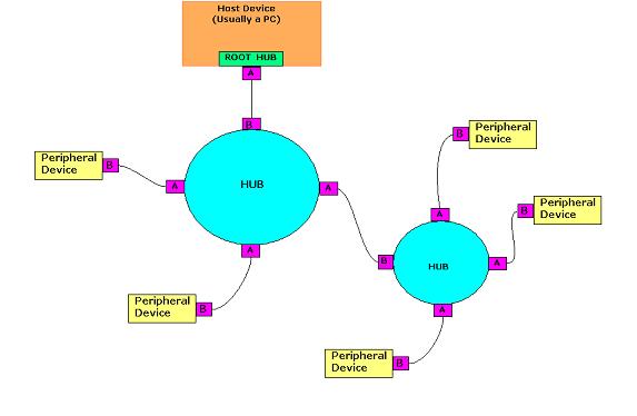 FIGURE
Fig2: The USB "tiered star"
topology
FIGURE
Fig2: The USB "tiered star"
topology
The hubs are bridges. They expand the logical and physical
fan-out of the network. A hub has a single upstream connection
(that going to the root hub, or the next hub closer to the
root), and one to many downstream connections.
Hubs themselves are considered as USB devices, and may
incorporate some amount of intelligence. We know that in
USB users may connect and remove peripherals without powering
the entire system down. Hubs detect these topology changes.
They also source power to the USB network. The power can
come from the hub itself (if it has a built-in power supply),
or can be passed through from an upstream hub.
USB connectors & the power supply:
Connecting a USB device to a computer is very simple -- you find the USB connector on the back of your machine and plug the USB connector into it. If it is a new device, the operating system auto-detects it and asks for the driver disk. If the device has already been installed, the computer activates it and starts talking to it.
Connecting a USB device to a computer is very simple -- you find the USB connector on the back of your machine and plug the USB connector into it. If it is a new device, the operating system auto-detects it and asks for the driver disk. If the device has already been installed, the computer activates it and starts talking to it.
The USB standard specifies two kinds of cables and connectors.
The USB cable will usually have an "A" connector
on one end and a "B" on the other. That means
the USB devices will have an "A" connection on
it. If not, then the device has a socket on it that accepts
a USB "B" connector.
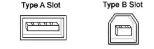
Fig 3: USB Type A
& B Connectors
The USB standard uses "A" and "B" connectors
mainly to avoid confusion:
1. "A" connectors head "upstream" toward
the computer.
2. "B" connectors head "downstream" and connect to individual devices.
2. "B" connectors head "downstream" and connect to individual devices.
By using different connectors on the upstream and downstream
end, it is impossible to install a cable incorrectly, because
the two types are physically different.
Individual USB cables can run as long as 5 meters for 12Mbps
connections and 3m for 1.5Mbps. With hubs, devices can be
up to 30 meters (six cables' worth) away from the host.
Here the high-speed cables for 12Mbps communication are
better shielded than their less expensive 1.5Mbps counterparts.
The USB 2.0 specification tells that the cable delay to
be less than 5.2 ns per meter
Inside the USB cable there are two wires that supply the
power to the peripherals-- +5 volts (red) and ground (brown)--
and a twisted pair (yellow and blue) of wires to carry the
data. On the power wires, the computer can supply up to
500 milliamps of power at 5 volts. A peripheral that draws
up to 100ma can extract all of its power from the bus wiring
all of the time. If the device needs more than a half-amp,
then it must have its own power supply. That means low-power
devices such as mice can draw their power directly from
the bus. High-power devices such as printers have their
own power supplies and draw minimal power from the bus.
Hubs can have their own power supplies to provide power
to devices connected to the hub.
| Pin No: | Signal | Color of the cable |
| 1 | +5V power | Red |
| 2 | - Data | White / Yellow |
| 3 | +Data | Green / Blue |
| 4 | Ground | Black/Brown |
Table - 1: USB pin connections
USB hosts and hubs manage power by enabling and disabling
power to individual devices to electrically remove ill-behaved
peripherals from the system. Further, they can instruct
devices to enter the suspend state, which reduces maximum
power consumption to 500 microamps (for low-power, 1.5Mbps
peripherals) or 2.5ma for 12Mbps devices.
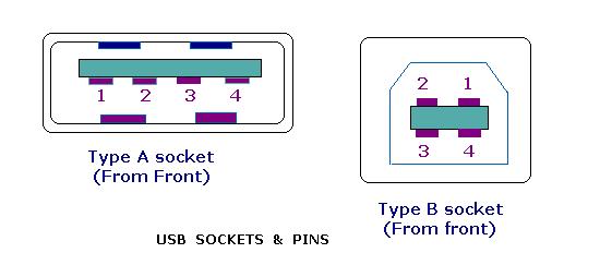
Fig 3: USB Type A & B Connectors
In short, the USB is a serial protocol and physical link,
which transmits all data differentially on a single pair
of wires. Another pair provides power to downstream peripherals.
Note that although USB cables having a Type A plug at each
end are available, they should never be used to connect
two PCs together, via their USB ports. This is because a
USB network can only have one host, and both would try to
claim that role. In any case, the cable would also short
their 5V power rails together, which could cause a damaging
current to flow. USB is not designed for direct data transfer
between PCs.
But the "sharing hubs" technique allows multiple computers to access the same peripheral device(s) and work by switching access between PCs, either automatically or manually.
But the "sharing hubs" technique allows multiple computers to access the same peripheral device(s) and work by switching access between PCs, either automatically or manually.
USB Electrical signaling
The serial data is sent along the USB in differential or
push-pull mode, with opposite polarities on the two signal
lines. This improves the signal-to-noise ratio by doubling
the effective signal amplitude and also allowing the cancellation
of any common-mode noise induced into the cable. The data
is sent in non-return-to-zero (NRTZ) format. To ensure a
minimum density of signal transitions, USB uses bit stuffing.
I.e.: an extra 0 bit is inserted into the data stream after
any appearance of six consecutive 1 bits. Seven consecutive
1 bits is always considered as an error.
The low speed/full speed USB bus (twisted pair data cable)
has characteristic impedance of 90 ohms +/- 15%. The data
cable signal lines are labeled as D+ and D-. Transmitted
signal levels are as follows.
1. 0.0V to 0.3V for low level and 2.8V to 3.6V for high
level in Full Speed (FS) and Low Speed (LS) modes
2. -10mV to 10 mV for low level and 360mV to 440 mV for high level in High Speed (HS) mode.
2. -10mV to 10 mV for low level and 360mV to 440 mV for high level in High Speed (HS) mode.
In FS mode the cable wires are not terminated, but the
HS mode has termination of 45O to ground, or 90O differential
to match the data cable impedance.
As we already discussed, the USB connection is always between
a host / hub at the "A" connector end, and a device
or hub's upstream port at the other end. The host includes
15 kO pull-down resistors on each data line. When no device
is connected, this pulls both data lines low into the so-called
"single-ended zero" state (SE0), and indicates
a reset or disconnected connection.
A USB device pulls one of the data lines high with a 1.5kO
resistor. This overpowers one of the pull-down resistors
in the host and leaves the data lines in an idle state called
"J". The choice of data line indicates a device's
speed support; full-speed devices pull D+ high, while low-speed
devices pull D- high. In fact the data is transmitted by
toggling the data lines between the J state and the opposite
K state.
A USB bus is reset using a prolonged (10 to 20 milliseconds)
SE0 signal. USB 2.0 devices use a special protocol during
reset, called "chirping", to negotiate the High-Speed
mode with the host/hub. A device that is HS capable first
connects as an FS device (D+ pulled high), but upon receiving
a USB RESET (both D+ and D- driven LOW by host for 10 to
20 mS) it pulls the D- line high. If the host/hub is also
HS capable, it chirps (returns alternating J and K states
on D- and D+ lines) letting the device know that the hub
will operate at High Speed.
How do they communicate?
When a USB peripheral device is first attached to the network,
a process called enumeration process gets started. This
is the way by which the host communicates with the device
to learn its identity and to discover which device driver
is required. The enumeration starts by sending a reset signal
to the newly connected USB device. The speed of the USB
device is determined during the reset signaling. After reset,
the host reads the USB device's information, and then the
device is assigned a unique 7-bit address (will be discussed
in next section). This avoids the DIP-switch and IRQ headaches
of the past device communication methods. If the device
is supported by the host, the device drivers needed for
communicating with the device are loaded and the device
is set to a configured state. Once a hub detects a new peripheral
(or even the removal of one), it actually reports the new
information about the peripheral to the host, and enables
communications with it. If the USB host is restarted, the
enumeration process is repeated for all connected devices.
In other words, the enumeration process is initiated both
when the host is powered up and a device connected or removed
from the network.
Technically speaking, the USB communications takes place
between the host and endpoints located in the peripherals.
An endpoint is a uniquely addressable portion of the peripheral
that is the source or receiver of data. Four bits define
the device's endpoint address; codes also indicate transfer
direction and whether the transaction is a "control"
transfer (will be discussed later in detail). Endpoint 0
is reserved for control transfers, leaving up to 15 bi-directional
destinations or sources of data within each device. All
devices must support endpoint zero. Because this is the
endpoint, which receives all of the devices control, and
status requests during enumeration and throughout the duration
while the device is operational on the bus.
All the transfers in USB occur through virtual pipes that
connect the peripheral's endpoints with the host. When establishing
communications with the peripheral, each endpoint returns
a descriptor, a data structure that tells the host about
the endpoint's configuration and expectations. Descriptors
include transfer type, max size of data packets, perhaps
the interval for data transfers, and in some cases, the
bandwidth needed. Given this data, the host establishes
connections to the endpoints through virtual pipes.
Though physically configured as a tiered star, logically
(to the application code) a direct connection exists between
the host and each device.
The host controller polls the bus for traffic, usually
in a round-robin fashion, so no USB device can transfer
any data on the bus without an explicit request from the
host controller.
USB can support four data transfer types or transfer mode,
which are listed below.
1. Control
2. Isochronous
3. Bulk
4. Interrupt
1. Control
2. Isochronous
3. Bulk
4. Interrupt
Control transfers exchange configuration, setup and command
information between the device and the host. The host can
also send commands or query parameters with control packets.
Isochronous transfer is used by time critical, streaming
device such as speakers and video cameras. It is time sensitive
information so, within limitations, it has guaranteed access
to the USB bus. Data streams between the device and the
host in real-time, and so there will not be any error correction.
Bulk transfer is used by device like printers & scanners,
which receives data in one big packet. Here the timely delivery
is not critical. Bulk transfers are fillers, claiming unused
USB bandwidth when nothing more important is going on. The
error correction protects these packets.
Interrupt transfers is used by peripherals exchanging small
amounts of data that need immediate attention. It is used
by devices to request servicing from the PC/host. Devices
like a mouse or a keyboard comes in this category. Error
checking validates the data.
As devices are enumerated, the host is keeping track of
the total bandwidth that all of the isochronous and interrupt
devices are requesting. They can consume up to 90 percent
of the 480 Mbps of bandwidth that is available. After 90
percent is used up, the host denies access to any other
isochronous or interrupt devices. Control packets and packets
for bulk transfers use any bandwidth left over (at least
10 percent).
The USB divides the available bandwidth into frames, and
the host controls the frames. Frames contain 1,500 bytes,
and a new frame starts every millisecond. During a frame,
isochronous and interrupt devices get a slot so they are
guaranteed the bandwidth they need. Bulk and control transfers
use whatever space is left.
USB packets & formats
All USB data is sent serially, of course, and least significant
bit (LSB) first. USB data transfer is essentially in the
form of packets of data, sent back and forth between the
host and peripheral devices. Initially, all packets are
sent from the host, via the root hub and possibly more hubs,
to devices. Some of those packets direct a device to send
some packets in reply.
Each USB data transfer consists of a
1. Token Packet (Header defining what it expects to follow)
2. Optional Data Packet, (Containing the payload)
3. Status Packet (Used to acknowledge transactions and to provide a means of error correction)
2. Optional Data Packet, (Containing the payload)
3. Status Packet (Used to acknowledge transactions and to provide a means of error correction)
As we have already discussed, the host initiates all transactions.
The first packet, also called a token is generated by the
host to describe what is to follow and whether the data
transfer will be a read or write and what the device's address
and designated endpoint is. The next packet is generally
a data packet carrying the content information and is followed
by a handshaking packet, reporting if the data or token
was received successfully, or if the endpoint is stalled
or not available to accept data.
USB packets may consist of the following fields:
1. Sync field: All the packets start with this sync field.
The sync field is 8 bits long at low and full speed or 32
bits long for high speed and is used to synchronize the
clock of the receiver with that of the transmitter. The
last two bits indicate where the PID fields starts.
2. PID field: This field (Packet ID) is used to identify
the type of packet that is being sent. The PID is actually
4 bits; the byte consists of the 4-bit PID followed by its
bit-wise complement, making an 8-bit PID in total. This
redundancy helps detect errors.
3. ADDR field: The address field specifies which device
the packet is designated for. Being 7 bits in length allows
for 127 devices to be supported.
4. ENDP field: This field is made up of 4 bits, allowing
16 possible endpoints. Low speed devices however can only
have 2 additional endpoints on top of the default pipe.
5. CRC field: Cyclic Redundancy Checks are performed on
the data within the packet payload. All token packets have
a 5-bit CRC while data packets have a 16-bit CRC.
6. EOP field: This indicates End of packet. Signaled by
a Single Ended Zero (SE0) for approximately 2 bit times
followed by a J for 1 bit time.
The USB packets come in four basic types, each with a different
format and CRC field:
1. Handshake packets
2. Token packets
3. Data packets
4. PRE packet
5. Start of Frame Packets
2. Token packets
3. Data packets
4. PRE packet
5. Start of Frame Packets
Handshake packets:
Handshake packets consist of a PID byte, and are generally
sent in response to data packets. The three basic types
of handshake packets are
1. ACK, indicating that data was successfully received,
2. NAK, indicating that the data cannot be received at this time and should be retried,
3. STALL, indicating that the device has an error and will never be able to successfully transfer data until some corrective action is performed.
2. NAK, indicating that the data cannot be received at this time and should be retried,
3. STALL, indicating that the device has an error and will never be able to successfully transfer data until some corrective action is performed.
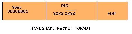
Fig 4: Handshake packet
format
USB 2.0 added two additional handshake packets.
1. NYET which indicates that a split transaction is not
yet complete,
2. ERR handshake to indicate that a split transaction failed.
2. ERR handshake to indicate that a split transaction failed.
The only handshake packet the USB host may generate is
ACK; if it is not ready to receive data, it should not instruct
a device to send any.
Token packets:
Token packets consist of a PID byte followed by 11 bits
of address and a 5-bit CRC. Tokens are only sent by the
host, not by a device.
There are three types of token packets.
1. In token - Informs the USB device that the host wishes
to read information.
2. Out token- informs the USB device that the host wishes to send information.
3. Setup token - Used to begin control transfers.
2. Out token- informs the USB device that the host wishes to send information.
3. Setup token - Used to begin control transfers.
IN and OUT tokens contain a 7-bit device number and 4-bit
function number (for multifunction devices) and command
the device to transmit DATA-packets, or receive the following
DATA-packets, respectively.
An IN token expects a response from a device. The response
may be a NAK or STALL response, or a DATA frame. In the
latter case, the host issues an ACK handshake if appropriate.
An OUT token is followed immediately by a DATA frame. The
device responds with ACK, NAK, or STALL, as appropriate.
SETUP operates much like an OUT token, but is used for
initial device setup.
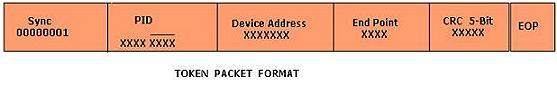
Fig 5: Token packet
format
USB 2.0 added a PING token, which asks a device if it is
ready to receive an OUT/DATA packet pair. The device responds
with ACK, NAK, or STALL, as appropriate. This avoids the
need to send the DATA packet if the device knows that it
will just respond with NAK.
USB 2.0 also added a larger SPLIT token with a 7-bit hub
number, 12 bits of control flags, and a 5-bit CRC. This
is used to perform split transactions. Rather than tie up
the high-speed USB bus sending data to a slower USB device,
the nearest high-speed capable hub receives a SPLIT token
followed by one or two USB packets at high speed, performs
the data transfer at full or low speed, and provides the
response at high speed when prompted by a second SPLIT token.
Data packets:
There are two basic data packets, DATA0 and DATA1. Both
consist of a DATA PID field, 0-1023 bytes of data payload
and a 16-bit CRC. They must always be preceded by an address
token, and are usually followed by a handshake token from
the receiver back to the transmitter.
1. Maximum data payload size for low-speed devices is 8
bytes.
2. Maximum data payload size for full-speed devices is 1023 bytes.
3. Maximum data payload size for high-speed devices is 1024 bytes.
4. Data must be sent in multiples of bytes
2. Maximum data payload size for full-speed devices is 1023 bytes.
3. Maximum data payload size for high-speed devices is 1024 bytes.
4. Data must be sent in multiples of bytes
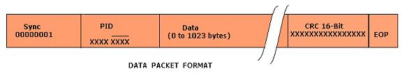
Fig6: Data packet
format
USB 2.0 added DATA2 and MDATA packet types as well. They
are used only by high-speed devices doing high-bandwidth
isochronous transfers, which need to transfer more than
1024 bytes per 125 µs "micro-frame" (8192
kB/s).
PRE packet:
Low-speed devices are supported with a special PID value,
PRE. This marks the beginning of a low-speed packet, and
is used by hubs, which normally do not send full-speed packets
to low-speed devices.
Since all PID bytes include four 0 bits, they leave the bus in the full-speed K state, which is the same as the low-speed J state. It is followed by a brief pause during which hubs enable their low-speed outputs, already idling in the J state, then a low-speed packet follows, beginning with a sync sequence and PID byte, and ending with a brief period of SE0. Full-speed devices other than hubs can simply ignore the PRE packet and its low-speed contents, until the final SE0 indicates that a new packet follows.
Since all PID bytes include four 0 bits, they leave the bus in the full-speed K state, which is the same as the low-speed J state. It is followed by a brief pause during which hubs enable their low-speed outputs, already idling in the J state, then a low-speed packet follows, beginning with a sync sequence and PID byte, and ending with a brief period of SE0. Full-speed devices other than hubs can simply ignore the PRE packet and its low-speed contents, until the final SE0 indicates that a new packet follows.
Start of Frame Packets:
Every 1ms (12000 full-speed bit times), the USB host transmits
a special SOF (start of frame) token, containing an 11-bit
incrementing frame number in place of a device address.
This is used to synchronize isochronous data flows. High-speed
USB 2.0 devices receive 7 additional duplicate SOF tokens
per frame, each introducing a 125 µs "micro-frame".
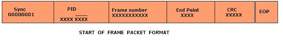
Fig7: Start of Frame
packet format
The Host controllers
As we know, the host controller and the root hub are part
of the computer hardware. The interfacing between the programmer
and this host controller is done by a device called Host
Controller Device (HCD), which is defined by the hardware
implementer.
In the version 1.x age, there were two competing HCD implementations,
Open Host Controller Interface (OHCI) and Universal Host
Controller Interface (UHCI). OHCI was developed by Compaq,
Microsoft and National Semiconductor. UHCI and its open
software stack were developed by Intel. VIA Technologies
licensed the UHCI standard from Intel; all other chipset
implementers use OHCI. UHCI is more software-driven, making
UHCI slightly more processor-intensive than OHCI but cheaper
to implement.
With the introduction of USB 2.0 a new Host Controller
Interface Specification was needed to describe the register
level details specific to USB 2.0. The USB 2.0 HCD implementation
is called the Enhanced Host Controller Interface (EHCI).
Only EHCI can support hi-speed (480 Mbit/s) transfers. Most
of PCI-based EHCI controllers contain other HCD implementations
called 'companion host controller' to support Full Speed
(12 Mbit/s) and may be used for any device that claims to
be a member of a certain class. An operating system is supposed
to implement all device classes so as to provide generic
drivers for any USB device.
But remember, USB specification does not specify any HCD
interfaces. The USB defines the format of data transfer
through the port, but not the system by which the USB hardware
communicates with the computer it sits in.
Device classes
USB defines class codes used to identify a device's functionality
and to load a device driver based on that functionality.
This enables a device driver writer to support devices from
different manufacturers that comply with a given class code.
There are two places on a device where class code information
can be placed. One place is in the Device Descriptor, and
the other is in Interface Descriptors. Some defined class
codes are allowed to be used only in a Device Descriptor,
others can be used in both Device and Interface Descriptors,
and some can only be used in Interface Descriptors.
Further developments in USB
USB OTG:
One of the biggest problems with USB is that its host controlled.
If we switch off a USB host, nothing else works. Also USB
does not support peer-to-peer communication. Let us take
an example: Many USB digital cameras can download data to
a PC, but it is unable to connect them directly to the USB
printer or to a CD Burner, something which is possible with
other communication mediums.
To combat these problems, a standard was created to USB
2.0. USB On-The-Go (OTG) was created in 2002. It is actually
a supplement to the USB 2.0 specification. USB OTG defines
a dual-role device, which can act as either a host or peripheral,
and can connect to a PC or other portable devices through
the same connector. The OTG specification details the "dual
role device", in which a device can function as both
a device controller (DC) and/or a host controller (HC).
The OTG host can have a targeted peripheral list. This
means the embedded device does not need to have a list of
every product and vendor ID or class driver. It can target
only one type of peripheral if needed.
Mini, Micro USBs
The OTG specification introduced two additional connectors.
One such connector is a mini A/B connector. A dual-role
device is required to be able to detect whether a Mini-A
or Mini-B plug is inserted by determining if the ID pin
(an extra pin introduced by OTG) is connected to ground.
The Standard-A plug is approximately 4 x 12 mm, the Standard-B
approximately 7 x 8 mm, and the Mini-A and Mini-B plugs
approximately 2 x 7 mm. These connectors are used for smaller
devices such as PDAs, mobile phones or digital cameras.
The Micro-USB connector was introduced in Jan-2007. It
was mainly intended to replace the Mini-USB plugs used in
many new smart-phones and PDAs. This Micro-USB plug is rated
for approximately 10,000 connect-disconnect cycles. As far
as the dimensions are concerned, it is about half the height
of the mini-USB connector, but features a similar width.
| Pin No: | Name | Description | Color |
| 1 | VCC | +5V | Red |
| 2 | D- | Data- | White |
| 3 | D+ | Data+ | Green |
| 4 | ID | Type –A: Connected to GNDType – B: Not connected | None |
| 5 | GND | Ground | Black |
With Courtesy :
http://www.eeherald.com/section/design-guide/esmod14.html
Subscribe to:
Posts (Atom)